Sep 7, 2026
Dynamic vs Static LCA in Circular Value Chains
Sustainability Strategy
In This Article
Timing decides if dynamic LCA is needed—use static for baselines and dynamic when delayed loops or grid shifts change outcomes.
Dynamic vs Static LCA in Circular Value Chains
If timing can change your result, static LCA is not enough. In circular value chains, products and materials can return years later through reuse, repair, remanufacturing, and recycling. That means the same product may face a different U.S. grid mix, fuel mix, and end-of-life system over time.
I’d sum it up like this:
Use static LCA when you need a baseline, a screen of options, or side-by-side reporting.
Use dynamic LCA when product life is long, loops happen years apart, or future conditions can shift the answer.
Use both for high-stakes choices: static for a common baseline, dynamic for timing risk.
A few numbers from the article make the point fast:
One building study found 25%–26% lower global warming results when it used a decarbonizing grid instead of a fixed grid.
One comparison found dynamic modeling at 3.57×10⁷ kg CO₂e, versus 1.07×10⁸ kg CO₂e in static modeling.
A packaging case found a bag with 80% recycled LDPE cut annual emissions by 191 t CO₂e versus the prior virgin LDPE bag.
What I take from this is simple: static LCA is best for consistency; dynamic LCA is best when timing drives the outcome. The choice depends on six things: time treatment, data needs, model effort, circular loop handling, future scenarios, and result comparability.
Quick Comparison
Factor | Static LCA | Dynamic LCA |
|---|---|---|
Time | One average view | Year-by-year view |
Data | Bills of materials, average electricity, transport, waste | Time-stamped energy, maintenance, lifetime, return, and recycling data |
Model effort | Lower | Higher |
Circular loops | Uses average loop effects | Separates loops by when they happen |
Future change | Limited | Includes grid, policy, and system shifts |
Best use | Baselines, screening, reporting | Long-life assets, delayed loops, carbon storage, policy planning |
If I were making the call, I’d start with one question: Will timing change which option wins? If the answer is no, static LCA is usually enough. If the answer is yes, dynamic LCA earns its place.
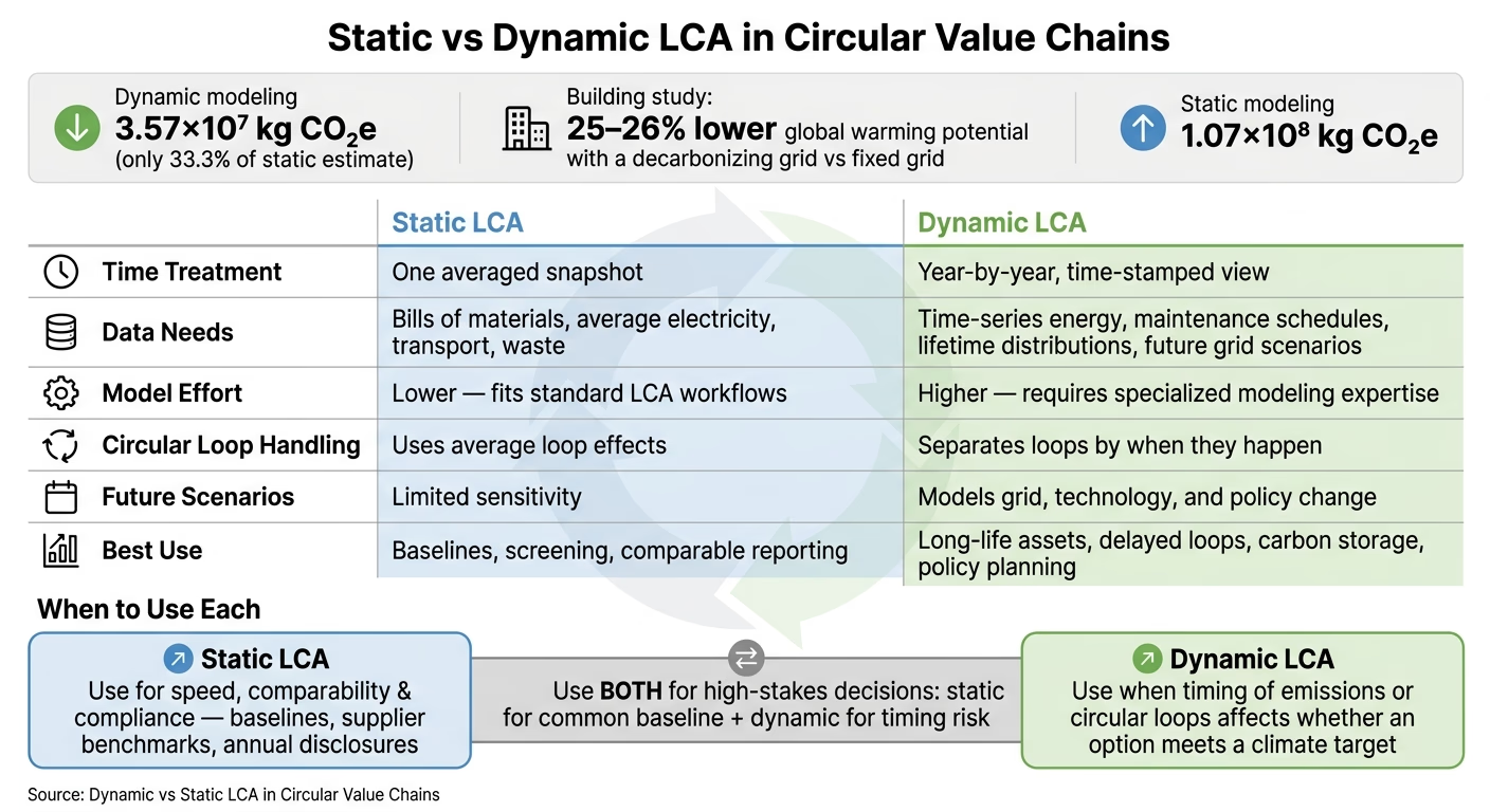
Static vs Dynamic LCA: Key Differences for Circular Value Chains
Dynamic LCA of an increased use of wood in buildings and its consequences- Sylvain Cordier-ACLCA2022
2. Static LCA: baselines, screening, and comparable reporting
Static LCA reduces a circular value chain to a single snapshot, using fixed assumptions and impact factors. That’s exactly why it’s practical. It skips future-year modeling and gives teams a straightforward way to compare circular options under current conditions. In practice, that makes static LCA the baseline method for circular comparisons.
2.1 Core assumptions, data needs, and system boundaries
Static LCA relies on average, fixed background data. In circular systems, that simplification helps when timing is not the main issue. Electricity, for example, is represented by the current regional grid mix. Transport is modeled with standard distances in miles and mode-specific data. Recycling rates are treated as constant.
To build a static LCA, a practitioner typically needs a bill of materials, electricity use, transport distances, waste flows, and recycled-content share. Those inputs are then matched with standard LCA databases to produce a footprint that is consistent and repeatable.
System boundaries matter because they determine what the model includes. Cradle-to-grave covers extraction through disposal. Cradle-to-cradle goes a step further by adding recycling loops and the avoided production of virgin material in the next cycle.
The recycling setup also changes the model:
In open-loop recycling, recovered materials move into a different product system. PET from beverage bottles recycled into textile fibers, for instance, can receive credits for displaced virgin polyester.
In closed-loop recycling, materials return to the same product system and are modeled with fixed average recycling rates and allocation rules.
If the boundary or allocation rule is vague, the comparison gets shaky fast. State both clearly so the results hold up.
2.2 Strengths and limits in circular systems
Static LCA’s biggest strength is access. It fits within the mature standards of ISO 14040 and ISO 14044, uses widely accepted characterization factors, and produces results that can be compared across products, suppliers, and portfolios.
For circular decisions, it works well as a screening and baseline tool. New Zealand Post commissioned a comparative packaging LCA and found that a courier bag made from 80% recycled LDPE outperformed five alternatives, reducing annual emissions by 191 t CO2e versus the original virgin LDPE bag.[1] That’s static LCA doing what it does best: ranking options, finding hotspots, and backing decisions based on current conditions.
Its limits show up when timing changes the result. Static LCA does not distinguish between an emission released today and one released years later under a different electricity mix. It treats temporary carbon storage the same as an immediate emission. It also assumes recycling rates stay fixed, even when a circular plan depends on increasing those rates over time.
That can be a big deal. For long-lived products, multi-cycle reuse systems, or strategies tied to grid decarbonization paths, the timing gap can shift the answer in a meaningful way.
Static LCA strengths | Static LCA weaknesses | Best-fit circular use cases |
|---|---|---|
Mature standards under ISO 14040/14044 | Does not model timing of emissions or environmental response | Product footprints and baseline reporting |
Lower modeling burden and cost | Can miss delayed emissions and temporary carbon storage | Packaging comparisons and reuse-vs-single-use screening |
Easier comparability when functional equivalence is defined | May blur impacts across multiple use cycles or dynamic recycling rates | Portfolio reviews and policy baselines |
Works with established databases and emission factors | Can understate or overstate impacts when future grid mixes or end-of-life pathways shift | Early-stage circular design decisions |
Static LCA is at its best when assumptions on recycled content, end-of-life routes, and allocation rules are explicit. Its main weak point is time: it flattens benefits and burdens that happen years apart.
3. Dynamic LCA: accounting for timing in circular decisions
Dynamic LCA brings time into both the inventory and the impact assessment. Instead of treating emissions, resource use, and background conditions as one fixed snapshot, it follows how they change over the study period. That includes shifts in the electricity grid, changes in recycling systems, and other moving parts that play out over years or even decades. In practice, it models emissions and material flows as time-based profiles, not one rolled-up total. That makes it most useful when future conditions drive the answer more than today’s averages.
This becomes especially important for long-lived systems and delayed circular loops. A building LCA study that compared static and dynamic electricity mix assumptions found an average 25–26% reduction in global warming potential when it used a gradually decarbonizing grid rather than a fixed current mix.[2] The same idea applies to delayed end-of-life effects, biogenic carbon storage, and long maintenance cycles. To do that well, you need inventory data with time stamps.
3.1 Dynamic inventory, dynamic impacts, and time boundaries
At the inventory stage, a dynamic life cycle inventory (DLCI) assigns a time stamp to each flow. It records flows year by year instead of lumping them into one total. Dynamic impact assessment (DLCIA) adds another layer by applying time-dependent characterization factors. For climate change, that means tracking how greenhouse gas concentrations and radiative forcing change over time, so an emission released early in the study period is judged differently from one released near the end. For toxicity, dynamic factors can show short-term exposure spikes that a static model would blur into an average.
It helps to keep two working ideas separate: the resolution used to record flows, and the full time horizon of the study. Annual time steps are often enough for climate work. Toxicity may call for finer intervals. The time horizon could be 30 years for a building or 60 years for infrastructure, and that choice can shift which option comes out ahead. In some dynamic models, even the system boundary changes over time. A model may bring in future reuse, remanufacturing, or secondary markets once they appear.
Fully dynamic LCA is still uncommon because it takes more time, data, and modeling effort. So in practice, many studies are only partly dynamic. A team might time-stamp operational energy and maintenance but keep static characterization factors for most impact categories. Or it might use a dynamic climate model while leaving other categories alone. For circular value chains, that kind of step-by-step approach can still matter a lot when the biggest time-sensitive drivers are grid decarbonization, biogenic carbon, and toxicity peaks.
3.2 Data needs, modeling tools, and practical limits
Dynamic LCA needs foreground data expressed over time, not just as totals. The key inputs usually include:
Use-phase energy profiles matched to projected grid mixes
Maintenance and replacement schedules
Product lifetime distributions
Time-dependent collection and recycling rates
Multi-decade profiles of biogenic carbon uptake, storage, and release
Tools like digital twins, IoT sensors, and system dynamics models make this much more workable. Digital twins - virtual replicas of physical assets - can produce high-resolution time series for energy use, throughput, and maintenance events across reuse and remanufacturing cycles. IoT sensors and smart meters add time-stamped data on consumption and degradation, showing how circular loops perform as time passes. System dynamics models can map feedback loops and changing stocks, such as growing pools of reusable products or larger recycling capacity, and turn those patterns into time-dependent material flows.
A practical way to start is simple: add temporal detail first to the foreground processes where timing has the biggest effect, especially use-phase energy, major maintenance, and end-of-life treatment. Then apply dynamic impact methods where established models already exist, especially for climate and key toxicity pathways. The upside is a clearer picture for time-sensitive decisions. The downside is a heavier modeling load.
Factor | Dynamic LCA | Static LCA |
|---|---|---|
Main limitation | Sensitive to the chosen time horizon; rankings can change | Misses timing-driven differences and flattens impacts across years |
Data requirements | Time-series energy use, maintenance schedules, lifetime distributions, future grid scenarios | Bill of materials, average electricity mix, standard transport, and waste data |
Resource intensity | High; specialized modeling expertise required | Moderate; fits standard LCA workflows |
Best uses | Long-lived assets, decarbonization planning, biogenic carbon, and multi-cycle reuse strategies | Screening, baseline reporting, and comparable reporting |
4. Dynamic vs. static LCA: where results diverge and which method fits
Timing can change the result in a big way. In one comparative analysis, dynamic modeling produced 3.57×10⁷ kg CO₂e, which was 33.3% of the static estimate of 1.07×10⁸ kg CO₂e.[6] That gap came from timing, not just from different system boundaries. In circular systems, delayed reuse and a changing grid can shift the outcome enough that a static estimate no longer tells the whole story.
4.1 Side-by-side comparison across six decision factors
The six factors below do most of the heavy lifting when you’re choosing a method. Put simply: they show when timing matters enough to make dynamic modeling worth the extra work.
Decision Factor | Static LCA | Dynamic LCA |
|---|---|---|
Treatment of time | One averaged point in time. | Timing is explicit. |
Data needs | Average database inputs. | Time-stamped operational and scenario data. |
Modeling complexity | Standard LCA workflow. | Time-dependent inventory and impact modeling. |
Handling of circular loops | Static averages loop effects. | Dynamic separates them by timing. |
Forward-looking scenarios | Limited scenario sensitivity. | Models grid, technology, and policy change. |
Result comparability | Easier to compare. | Scenario-specific. |
If circular loops are short and the decision horizon is near term, static LCA will usually give enough directional guidance. But when loops stretch over years, assets stay in service for a long time, or the grid is likely to change a lot, static results can gloss over timing effects that matter. That’s often where delayed emissions, carbon storage, or future low-carbon electricity start to shift the answer.
4.2 When to use each method for supply chain planning and policy work
Once the comparison is on the table, the next step is choosing the right fit.
Static LCA works well for baseline footprinting, procurement screening, and standardized reporting. It’s a good choice for screening, disclosure, and supplier comparisons, where consistency and side-by-side review matter most.
Dynamic LCA makes more sense when timing changes the answer in a material way. That often includes long-lived infrastructure, bio-based materials with carbon storage, and policy design where impacts unfold over time. In those cases, timing doesn’t just add detail - it changes the result.
For major capital projects, a paired approach often works best: use a static baseline for comparability, then add dynamic scenarios to test timing risk.
5. Conclusion: match the method to the decision, not the trend
Neither method is better in every case. Static LCA remains the right default for baseline footprinting, supplier screening, and comparable reporting across products, facilities, and years. It works well because it relies on fixed, time-aggregated inventories and standard methods. Dynamic LCA makes sense only when timing changes the outcome of the decision, such as with long-lived infrastructure, bio-based materials that store carbon, or policy choices tied to climate milestones like 2030 or 2050 targets.[4][7]
The simplest way to think about it is this: use static LCA for the baseline, then bring in dynamic analysis only when timing could change which option wins.
A few rules of thumb help keep that choice clear:
Use static LCA for speed, comparability, and compliance: baselines, supplier benchmarks, and annual disclosures.
Use dynamic LCA when the timing of emissions or circular loops affects whether a given option can meet a climate target.
Start from the decision: “Which option is better overall?” points to static. “When and how do impacts occur?” points to dynamic.
Match complexity to data quality. Do you have time-resolved flow data, known reuse cycles and return rates, and the tools and staff capacity to keep time-dependent inventories up to date? If the answer is mostly no, a strong static LCA is the more defensible choice.[4][5]
Layer the two methods: static for broad baselines, dynamic for high-stakes circular interventions, then refine over time as your data and internal capacity improve.[4][7][3]
This approach keeps the work tied to the decision that matters, instead of chasing the newest method for its own sake.
FAQs
How do I know if timing will change my LCA result?
Use a sensitivity analysis to test how changes in assumptions - including timing - affect your life cycle assessment results.
This matters because LCA results can shift a lot based on data quality and modeling choices. In circular value chains, material availability and energy grids don’t stay fixed over time. A check on these time-based variables helps keep your results accurate and useful for decision-making.
What data do I need before attempting a dynamic LCA?
Start by mapping material flows, setting clear system boundaries, and choosing a functional unit. That gives the assessment a firm frame before you get into the numbers. From there, collect life cycle inventory data for the main inputs and outputs, including raw materials, energy, water, emissions, and waste.
For the categories that matter most, lean on primary, supplier-specific data whenever you can. It gives you a closer view of what’s happening in the actual supply chain, not just a generic average. Just as important, write down your methods and assumptions as you go, and stick to one measurement system throughout. That makes the work easier to track, compare, and test through sensitivity analysis.
Can I combine static and dynamic LCA in one decision process?
Yes. Using both can make the decision process stronger.
Static LCA gives you a point-in-time view based on average data. Dynamic LCA adds the time dimension, showing how results shift as supply chain conditions, energy mixes, and production patterns change.
In practice, many teams split the work this way:
Static LCA for annual reporting, disclosures, and compliance
Dynamic LCA for higher-stakes choices such as material substitutions or process changes, where timing can affect supply chain planning and policy decisions
That setup gives you a steady baseline for reporting, while also giving decision-makers a sharper view when the choice on the table has moving parts.
Related Blog Posts
Latest Articles
©2026

Narrative Change and Power Building: The Missing Half of Advocacy
Narrative change is the process of disrupting dominant narratives that normalize inequity and advancing new narratives from historically marginalized communities.

Funding Resilience Without Federal Grants
BRIC is unreliable and FEMA is shrinking. Here's how cities fund climate resilience with dedicated revenue, blended finance, and a coordinating authority.

The ESG Blind Spot: How AI Is Finding Risks in Companies Nobody Else Is Watching
Norway's sovereign wealth fund uses AI to screen 7,200 portfolio companies for forced labor and corruption within 24 hours. The real story is the emerging-market coverage gap that traditional ESG data vendors miss — and what it means for any company with a global supply chain.
Narrative Change and Power Building: The Missing Half of Advocacy
Narrative change is the process of disrupting dominant narratives that normalize inequity and advancing new narratives from historically marginalized communities.
Funding Resilience Without Federal Grants
BRIC is unreliable and FEMA is shrinking. Here's how cities fund climate resilience with dedicated revenue, blended finance, and a coordinating authority.
The ESG Blind Spot: How AI Is Finding Risks in Companies Nobody Else Is Watching
Norway's sovereign wealth fund uses AI to screen 7,200 portfolio companies for forced labor and corruption within 24 hours. The real story is the emerging-market coverage gap that traditional ESG data vendors miss — and what it means for any company with a global supply chain.
FAQ
01
What does it really mean to “redefine profit”?
02
What makes Council Fire different?
03
Who does Council Fire work with?
04
What does working with Council Fire actually look like?
05
How does Council Fire help organizations turn big goals into action?
06
How does Council Fire define and measure success?
07
How does technology fit into Council Fire’s work?
Sep 7, 2026
Dynamic vs Static LCA in Circular Value Chains
Sustainability Strategy
In This Article
Timing decides if dynamic LCA is needed—use static for baselines and dynamic when delayed loops or grid shifts change outcomes.
Dynamic vs Static LCA in Circular Value Chains
If timing can change your result, static LCA is not enough. In circular value chains, products and materials can return years later through reuse, repair, remanufacturing, and recycling. That means the same product may face a different U.S. grid mix, fuel mix, and end-of-life system over time.
I’d sum it up like this:
Use static LCA when you need a baseline, a screen of options, or side-by-side reporting.
Use dynamic LCA when product life is long, loops happen years apart, or future conditions can shift the answer.
Use both for high-stakes choices: static for a common baseline, dynamic for timing risk.
A few numbers from the article make the point fast:
One building study found 25%–26% lower global warming results when it used a decarbonizing grid instead of a fixed grid.
One comparison found dynamic modeling at 3.57×10⁷ kg CO₂e, versus 1.07×10⁸ kg CO₂e in static modeling.
A packaging case found a bag with 80% recycled LDPE cut annual emissions by 191 t CO₂e versus the prior virgin LDPE bag.
What I take from this is simple: static LCA is best for consistency; dynamic LCA is best when timing drives the outcome. The choice depends on six things: time treatment, data needs, model effort, circular loop handling, future scenarios, and result comparability.
Quick Comparison
Factor | Static LCA | Dynamic LCA |
|---|---|---|
Time | One average view | Year-by-year view |
Data | Bills of materials, average electricity, transport, waste | Time-stamped energy, maintenance, lifetime, return, and recycling data |
Model effort | Lower | Higher |
Circular loops | Uses average loop effects | Separates loops by when they happen |
Future change | Limited | Includes grid, policy, and system shifts |
Best use | Baselines, screening, reporting | Long-life assets, delayed loops, carbon storage, policy planning |
If I were making the call, I’d start with one question: Will timing change which option wins? If the answer is no, static LCA is usually enough. If the answer is yes, dynamic LCA earns its place.
Static vs Dynamic LCA: Key Differences for Circular Value Chains
Dynamic LCA of an increased use of wood in buildings and its consequences- Sylvain Cordier-ACLCA2022
2. Static LCA: baselines, screening, and comparable reporting
Static LCA reduces a circular value chain to a single snapshot, using fixed assumptions and impact factors. That’s exactly why it’s practical. It skips future-year modeling and gives teams a straightforward way to compare circular options under current conditions. In practice, that makes static LCA the baseline method for circular comparisons.
2.1 Core assumptions, data needs, and system boundaries
Static LCA relies on average, fixed background data. In circular systems, that simplification helps when timing is not the main issue. Electricity, for example, is represented by the current regional grid mix. Transport is modeled with standard distances in miles and mode-specific data. Recycling rates are treated as constant.
To build a static LCA, a practitioner typically needs a bill of materials, electricity use, transport distances, waste flows, and recycled-content share. Those inputs are then matched with standard LCA databases to produce a footprint that is consistent and repeatable.
System boundaries matter because they determine what the model includes. Cradle-to-grave covers extraction through disposal. Cradle-to-cradle goes a step further by adding recycling loops and the avoided production of virgin material in the next cycle.
The recycling setup also changes the model:
In open-loop recycling, recovered materials move into a different product system. PET from beverage bottles recycled into textile fibers, for instance, can receive credits for displaced virgin polyester.
In closed-loop recycling, materials return to the same product system and are modeled with fixed average recycling rates and allocation rules.
If the boundary or allocation rule is vague, the comparison gets shaky fast. State both clearly so the results hold up.
2.2 Strengths and limits in circular systems
Static LCA’s biggest strength is access. It fits within the mature standards of ISO 14040 and ISO 14044, uses widely accepted characterization factors, and produces results that can be compared across products, suppliers, and portfolios.
For circular decisions, it works well as a screening and baseline tool. New Zealand Post commissioned a comparative packaging LCA and found that a courier bag made from 80% recycled LDPE outperformed five alternatives, reducing annual emissions by 191 t CO2e versus the original virgin LDPE bag.[1] That’s static LCA doing what it does best: ranking options, finding hotspots, and backing decisions based on current conditions.
Its limits show up when timing changes the result. Static LCA does not distinguish between an emission released today and one released years later under a different electricity mix. It treats temporary carbon storage the same as an immediate emission. It also assumes recycling rates stay fixed, even when a circular plan depends on increasing those rates over time.
That can be a big deal. For long-lived products, multi-cycle reuse systems, or strategies tied to grid decarbonization paths, the timing gap can shift the answer in a meaningful way.
Static LCA strengths | Static LCA weaknesses | Best-fit circular use cases |
|---|---|---|
Mature standards under ISO 14040/14044 | Does not model timing of emissions or environmental response | Product footprints and baseline reporting |
Lower modeling burden and cost | Can miss delayed emissions and temporary carbon storage | Packaging comparisons and reuse-vs-single-use screening |
Easier comparability when functional equivalence is defined | May blur impacts across multiple use cycles or dynamic recycling rates | Portfolio reviews and policy baselines |
Works with established databases and emission factors | Can understate or overstate impacts when future grid mixes or end-of-life pathways shift | Early-stage circular design decisions |
Static LCA is at its best when assumptions on recycled content, end-of-life routes, and allocation rules are explicit. Its main weak point is time: it flattens benefits and burdens that happen years apart.
3. Dynamic LCA: accounting for timing in circular decisions
Dynamic LCA brings time into both the inventory and the impact assessment. Instead of treating emissions, resource use, and background conditions as one fixed snapshot, it follows how they change over the study period. That includes shifts in the electricity grid, changes in recycling systems, and other moving parts that play out over years or even decades. In practice, it models emissions and material flows as time-based profiles, not one rolled-up total. That makes it most useful when future conditions drive the answer more than today’s averages.
This becomes especially important for long-lived systems and delayed circular loops. A building LCA study that compared static and dynamic electricity mix assumptions found an average 25–26% reduction in global warming potential when it used a gradually decarbonizing grid rather than a fixed current mix.[2] The same idea applies to delayed end-of-life effects, biogenic carbon storage, and long maintenance cycles. To do that well, you need inventory data with time stamps.
3.1 Dynamic inventory, dynamic impacts, and time boundaries
At the inventory stage, a dynamic life cycle inventory (DLCI) assigns a time stamp to each flow. It records flows year by year instead of lumping them into one total. Dynamic impact assessment (DLCIA) adds another layer by applying time-dependent characterization factors. For climate change, that means tracking how greenhouse gas concentrations and radiative forcing change over time, so an emission released early in the study period is judged differently from one released near the end. For toxicity, dynamic factors can show short-term exposure spikes that a static model would blur into an average.
It helps to keep two working ideas separate: the resolution used to record flows, and the full time horizon of the study. Annual time steps are often enough for climate work. Toxicity may call for finer intervals. The time horizon could be 30 years for a building or 60 years for infrastructure, and that choice can shift which option comes out ahead. In some dynamic models, even the system boundary changes over time. A model may bring in future reuse, remanufacturing, or secondary markets once they appear.
Fully dynamic LCA is still uncommon because it takes more time, data, and modeling effort. So in practice, many studies are only partly dynamic. A team might time-stamp operational energy and maintenance but keep static characterization factors for most impact categories. Or it might use a dynamic climate model while leaving other categories alone. For circular value chains, that kind of step-by-step approach can still matter a lot when the biggest time-sensitive drivers are grid decarbonization, biogenic carbon, and toxicity peaks.
3.2 Data needs, modeling tools, and practical limits
Dynamic LCA needs foreground data expressed over time, not just as totals. The key inputs usually include:
Use-phase energy profiles matched to projected grid mixes
Maintenance and replacement schedules
Product lifetime distributions
Time-dependent collection and recycling rates
Multi-decade profiles of biogenic carbon uptake, storage, and release
Tools like digital twins, IoT sensors, and system dynamics models make this much more workable. Digital twins - virtual replicas of physical assets - can produce high-resolution time series for energy use, throughput, and maintenance events across reuse and remanufacturing cycles. IoT sensors and smart meters add time-stamped data on consumption and degradation, showing how circular loops perform as time passes. System dynamics models can map feedback loops and changing stocks, such as growing pools of reusable products or larger recycling capacity, and turn those patterns into time-dependent material flows.
A practical way to start is simple: add temporal detail first to the foreground processes where timing has the biggest effect, especially use-phase energy, major maintenance, and end-of-life treatment. Then apply dynamic impact methods where established models already exist, especially for climate and key toxicity pathways. The upside is a clearer picture for time-sensitive decisions. The downside is a heavier modeling load.
Factor | Dynamic LCA | Static LCA |
|---|---|---|
Main limitation | Sensitive to the chosen time horizon; rankings can change | Misses timing-driven differences and flattens impacts across years |
Data requirements | Time-series energy use, maintenance schedules, lifetime distributions, future grid scenarios | Bill of materials, average electricity mix, standard transport, and waste data |
Resource intensity | High; specialized modeling expertise required | Moderate; fits standard LCA workflows |
Best uses | Long-lived assets, decarbonization planning, biogenic carbon, and multi-cycle reuse strategies | Screening, baseline reporting, and comparable reporting |
4. Dynamic vs. static LCA: where results diverge and which method fits
Timing can change the result in a big way. In one comparative analysis, dynamic modeling produced 3.57×10⁷ kg CO₂e, which was 33.3% of the static estimate of 1.07×10⁸ kg CO₂e.[6] That gap came from timing, not just from different system boundaries. In circular systems, delayed reuse and a changing grid can shift the outcome enough that a static estimate no longer tells the whole story.
4.1 Side-by-side comparison across six decision factors
The six factors below do most of the heavy lifting when you’re choosing a method. Put simply: they show when timing matters enough to make dynamic modeling worth the extra work.
Decision Factor | Static LCA | Dynamic LCA |
|---|---|---|
Treatment of time | One averaged point in time. | Timing is explicit. |
Data needs | Average database inputs. | Time-stamped operational and scenario data. |
Modeling complexity | Standard LCA workflow. | Time-dependent inventory and impact modeling. |
Handling of circular loops | Static averages loop effects. | Dynamic separates them by timing. |
Forward-looking scenarios | Limited scenario sensitivity. | Models grid, technology, and policy change. |
Result comparability | Easier to compare. | Scenario-specific. |
If circular loops are short and the decision horizon is near term, static LCA will usually give enough directional guidance. But when loops stretch over years, assets stay in service for a long time, or the grid is likely to change a lot, static results can gloss over timing effects that matter. That’s often where delayed emissions, carbon storage, or future low-carbon electricity start to shift the answer.
4.2 When to use each method for supply chain planning and policy work
Once the comparison is on the table, the next step is choosing the right fit.
Static LCA works well for baseline footprinting, procurement screening, and standardized reporting. It’s a good choice for screening, disclosure, and supplier comparisons, where consistency and side-by-side review matter most.
Dynamic LCA makes more sense when timing changes the answer in a material way. That often includes long-lived infrastructure, bio-based materials with carbon storage, and policy design where impacts unfold over time. In those cases, timing doesn’t just add detail - it changes the result.
For major capital projects, a paired approach often works best: use a static baseline for comparability, then add dynamic scenarios to test timing risk.
5. Conclusion: match the method to the decision, not the trend
Neither method is better in every case. Static LCA remains the right default for baseline footprinting, supplier screening, and comparable reporting across products, facilities, and years. It works well because it relies on fixed, time-aggregated inventories and standard methods. Dynamic LCA makes sense only when timing changes the outcome of the decision, such as with long-lived infrastructure, bio-based materials that store carbon, or policy choices tied to climate milestones like 2030 or 2050 targets.[4][7]
The simplest way to think about it is this: use static LCA for the baseline, then bring in dynamic analysis only when timing could change which option wins.
A few rules of thumb help keep that choice clear:
Use static LCA for speed, comparability, and compliance: baselines, supplier benchmarks, and annual disclosures.
Use dynamic LCA when the timing of emissions or circular loops affects whether a given option can meet a climate target.
Start from the decision: “Which option is better overall?” points to static. “When and how do impacts occur?” points to dynamic.
Match complexity to data quality. Do you have time-resolved flow data, known reuse cycles and return rates, and the tools and staff capacity to keep time-dependent inventories up to date? If the answer is mostly no, a strong static LCA is the more defensible choice.[4][5]
Layer the two methods: static for broad baselines, dynamic for high-stakes circular interventions, then refine over time as your data and internal capacity improve.[4][7][3]
This approach keeps the work tied to the decision that matters, instead of chasing the newest method for its own sake.
FAQs
How do I know if timing will change my LCA result?
Use a sensitivity analysis to test how changes in assumptions - including timing - affect your life cycle assessment results.
This matters because LCA results can shift a lot based on data quality and modeling choices. In circular value chains, material availability and energy grids don’t stay fixed over time. A check on these time-based variables helps keep your results accurate and useful for decision-making.
What data do I need before attempting a dynamic LCA?
Start by mapping material flows, setting clear system boundaries, and choosing a functional unit. That gives the assessment a firm frame before you get into the numbers. From there, collect life cycle inventory data for the main inputs and outputs, including raw materials, energy, water, emissions, and waste.
For the categories that matter most, lean on primary, supplier-specific data whenever you can. It gives you a closer view of what’s happening in the actual supply chain, not just a generic average. Just as important, write down your methods and assumptions as you go, and stick to one measurement system throughout. That makes the work easier to track, compare, and test through sensitivity analysis.
Can I combine static and dynamic LCA in one decision process?
Yes. Using both can make the decision process stronger.
Static LCA gives you a point-in-time view based on average data. Dynamic LCA adds the time dimension, showing how results shift as supply chain conditions, energy mixes, and production patterns change.
In practice, many teams split the work this way:
Static LCA for annual reporting, disclosures, and compliance
Dynamic LCA for higher-stakes choices such as material substitutions or process changes, where timing can affect supply chain planning and policy decisions
That setup gives you a steady baseline for reporting, while also giving decision-makers a sharper view when the choice on the table has moving parts.
Related Blog Posts
Latest Articles
©2026
Narrative Change and Power Building: The Missing Half of Advocacy
Narrative change is the process of disrupting dominant narratives that normalize inequity and advancing new narratives from historically marginalized communities.
Funding Resilience Without Federal Grants
BRIC is unreliable and FEMA is shrinking. Here's how cities fund climate resilience with dedicated revenue, blended finance, and a coordinating authority.
The ESG Blind Spot: How AI Is Finding Risks in Companies Nobody Else Is Watching
Norway's sovereign wealth fund uses AI to screen 7,200 portfolio companies for forced labor and corruption within 24 hours. The real story is the emerging-market coverage gap that traditional ESG data vendors miss — and what it means for any company with a global supply chain.
FAQ
What does it really mean to “redefine profit”?
What makes Council Fire different?
Who does Council Fire work with?
What does working with Council Fire actually look like?
How does Council Fire help organizations turn big goals into action?
How does Council Fire define and measure success?
How does technology fit into Council Fire’s work?