
Sep 8, 2026
Smart Meter Analytics for Energy Demand Planning
Sustainability Strategy
In This Article
Leverage 15-minute AMI reads to clean data, create load profiles, forecast peaks, and target TOU/DR programs by asset and segment.
Smart Meter Analytics for Energy Demand Planning
If your meter data is clean, you can plan demand with far less guesswork. With 15-minute or hourly AMI data, I can see peak hours, sort customers by load shape, forecast stress on feeders and transformers, and match programs like TOU rates, EV charging control, and thermostat cycling to the places they fit best.
By December 2023, U.S. utilities had installed 128.4 million advanced meters, covering 76.8% of the nation’s 167.2 million meters. That means this is no longer a niche planning tool. It is now a standard way to use interval data for grid and community energy decisions. This data-driven approach is a cornerstone of building climate resilience for modern infrastructure.
Here’s the article in plain terms:
Start with data quality. Use 12–24 months of interval reads, fix gaps, duplicate records, outliers, and DST errors.
Build load profiles. Separate homes, offices, industrial sites, campuses, and public facilities by how they use power across the day and year.
Forecast demand. Use short-, medium-, and long-range models to estimate load growth and stress periods.
Find peak trouble spots. Map peaks to hours, feeders, transformers, and substations, not just system totals.
Turn analysis into action. Use meter data to guide TOU pricing, peak-time rebates, direct load control, and community program targeting.
Check results. Compare pre- and post-program interval data to measure peak kW changes, bill effects, and who actually took part.
A few numbers show why this matters. One TOU pilot cut peak demand by 0.17 kW per customer. An Oklahoma project using dynamic pricing and smart thermostats cut peak demand by about 30%, or roughly 1.3 kW per customer. In Ontario, Peak Perks enrolled 200,000+ residents and delivered up to 187 MW of one-hour peak reduction.
I’d sum it up this way: clean meter data helps you find the right peak problem, in the right place, at the right hour, and then pick the right program to deal with it.
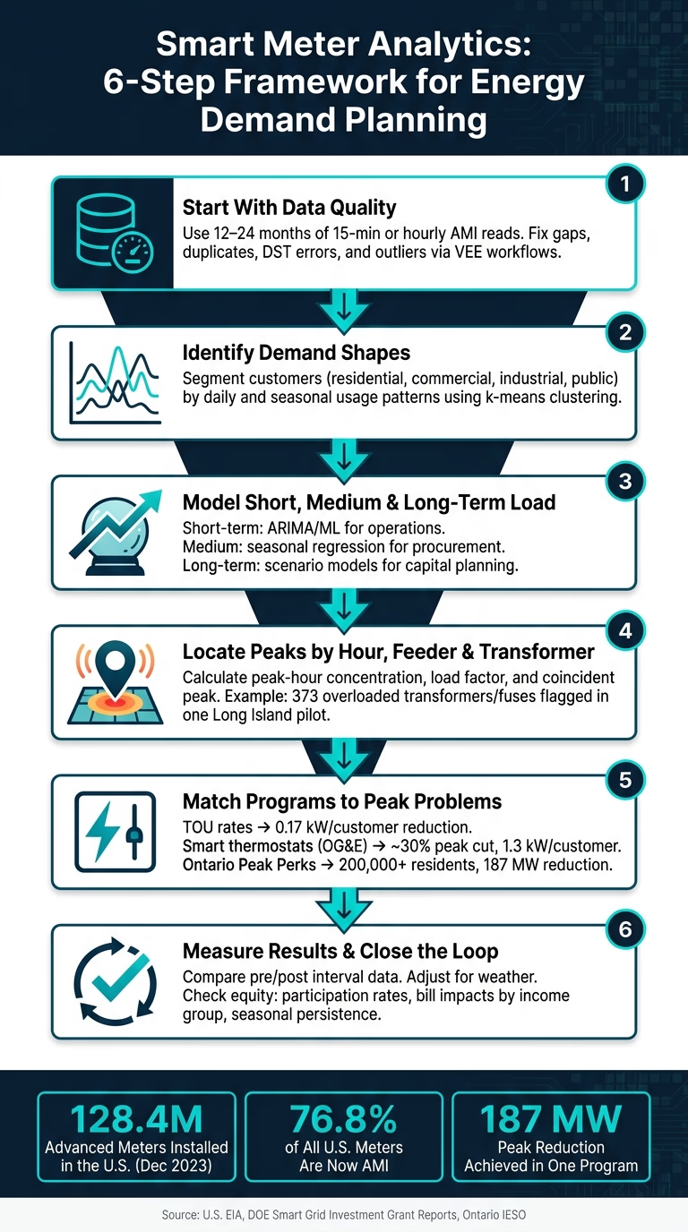
Smart Meter Analytics: 6-Step Framework for Energy Demand Planning
CCAI April Webinar: Smart Meter Data Analytics
Start With Smart Meter Data Collection and Quality Checks
Before any modeling starts, make sure AMI interval data is complete, accurate, and time-stamped the right way. Raw field data is messy more often than people expect. You’ll see gaps, duplicate reads, timestamp mistakes, and short spikes that don’t match actual usage. If that base layer is weak, everything built on top of it gets shaky fast. It starts with a clear planning dataset.
Define the Minimum Planning Dataset
Use 12 to 24 months of 15-minute or hourly kWh reads per meter. That time span is long enough to show daily load shapes, weekday-versus-weekend shifts, and seasonal patterns.
The dataset should include:
Meter ID
Customer account
Service address tied to feeder, transformer, or substation
Customer class, such as residential, small commercial, or industrial
Without those fields, it becomes almost impossible to tie demand patterns back to grid assets or customer segments.
Date and time stamps need to reflect local U.S. time, with daylight saving time (DST) handled correctly for each service territory. A one-hour timestamp shift might sound small, but it can push an apparent peak into the wrong time-of-use window and distort TOU analysis.
Weather, calendar, and building data help explain why load changes. Hourly temperature and humidity from nearby weather stations are especially useful for HVAC-driven demand, often measured through cooling degree days (CDD) and heating degree days (HDD). Building type, floor area, occupancy patterns, insulation levels, and whether the site has rooftop solar or EV chargers add context that interval reads alone can’t show. Calendar markers such as holidays, school days, weekends, and business hours also help surface repeat behavior.
Clean Timestamps, Gaps, Duplicates, and Outliers
Utilities usually run interval data through Validation, Editing, and Estimation (VEE) inside meter data management systems. VEE checks reads against set rules, flags bad values, and fills in missing intervals. For example, New York state MDMS rules estimate missing reads by averaging daily consumption from the same day of the week over the prior 45 days.[2] That kind of structured workflow keeps planning data consistent and defensible.
Here’s how the most common data issues show up in planning work:
Data-Quality Issue | Planning Impact | Typical Fix |
|---|---|---|
Missing intervals (gaps) | Underestimated peaks; biased load profiles; weak demand response sizing | Interpolate short gaps; exclude or model long gaps; monitor communications |
Time zone / DST errors | Misaligned peaks; incorrect TOU billing; flawed event analysis | Standardize to UTC with local mapping; apply DST rules consistently |
Duplicate records | Overstated consumption; inflated revenue and budget forecasts | De-duplicate by meter ID and timestamp; reconcile against billing totals |
Outliers / abnormal spikes | Exaggerated capacity needs; misleading program impact estimates | Flag with interquartile-range or z-score checks; cross-check against weather and system logs; cap or reconstruct confirmed meter errors |
This cleaning work is what makes later demand profiles and peak forecasts worth trusting. If the cleanup is sloppy, the planning mistakes can get expensive in a hurry. Overstated peaks can lead to unneeded infrastructure spending. Understated peaks can leave a grid segment short on capacity at the worst possible time. For filings such as integrated resource plans or rate cases, document completeness thresholds and imputation rules.[3]
Once the data is clean, it can feed load profiling, forecasting, and peak planning. The next step is to build load profiles and group customers by demand behavior.
Build Load Profiles and Group Customers by Demand Behavior
Clean interval data starts to pay off when you turn it into load profiles. That’s where raw meter reads become something planners can use. A hospital that runs 24/7 does not behave like a school that winds down in the afternoon, and if both get folded into the same demand plan, the result is predictable: poor timing on infrastructure, rate designs that miss the mark, and program dollars spent in the wrong places. Once those usage shapes come into focus, planners can forecast demand with more precision and see where peak strain is starting to build.
Identify Daily and Seasonal Demand Shapes
Cleaned interval data makes recurring patterns easy to spot across customer classes. Residential customers often show a morning ramp, a midday dip when people are out, and then a sharp evening peak from 5–9 p.m. when households come back, cook dinner, and switch on appliances. Commercial and office buildings tend to show the opposite pattern, with strong demand from 8 a.m.–5 p.m., a steady midday plateau, and a steep drop once the workday ends.
Seasonal swings matter just as much as daily ones. In summer, air conditioning pushes up residential and commercial demand, especially in the Southeast and Southwest, where late-afternoon peaks from 3–7 p.m. can put feeders under strain on the hottest days. As electrification grows, with more heat pumps and EVs on the system, winter load shapes are changing too. In colder regions, planners are seeing earlier morning peaks and a second spike in the evening. In transformer load modeling, winter heat pump profiles were split into four clusters, and one cluster represented about 64% of customers.[5]
Weather and calendar inputs make these profiles sharper. Temperature, humidity, and solar irradiance help separate HVAC-driven demand from steady baseload. Weekday versus weekend patterns, holidays, and school terms add another layer, which helps planners see whether a spike came from weather, occupancy, or both.
Use Segmentation to Find Planning-Relevant Customer Groups
Segmentation puts customers with similar demand shapes into segment profiles that utilities and planners can act on. The usual approach is simple: normalize daily load curves, then cluster them with methods like k-means or hierarchical clustering.
A large Illinois study looked at 2.5 million residential customers and used k-means clustering to sort them into six distinct load profiles, from flat usage to high-peak behavior. Flatter profiles showed up more often in urban and lower-income areas, while high-volume, sharply peaked demand was more common in higher-income suburban areas.[4] That kind of split is not just interesting on paper. It ties straight into infrastructure and program decisions.
Segment | Typical Load Shape | Planning Use |
|---|---|---|
Evening-peak households | Low daytime load, sharp 5–9 p.m. peak | Residential DR targeting, TOU rate design |
Office/weekday commercial | Strong 8 a.m.–5 p.m. load, low weekends | Summer afternoon DR events, distribution planning |
All-day residential | Higher daytime usage (work-from-home, multi-family) | Midday solar integration, EV charging programs |
24/7 industrial or data centers | High nighttime baseload, minimal weekday/weekend difference | Baseload capacity planning, demand response targeting |
Public lighting and facilities | Pronounced nighttime usage, seasonal daylight variation | Winter peak planning, lighting efficiency programs |
Each segment profile gives planners a practical way to test scenarios, estimate how much each group adds to system peaks, and shape outreach or incentives around how customers actually use power, not how planners assume they do. For community energy programs like neighborhood solar, resilience hubs, or local storage, segmentation helps match spending to the way power is used in a given area. These profiles then feed into demand forecasts and help flag the hours when the system is under the most pressure.
Forecast Demand and Locate Peak Stress Periods
Once segments are in place, meter data starts to show where peak stress is likely to show up first. Cleaned, segmented meter data surfaces demand at the circuit, feeder, neighborhood, and campus levels - places where system-wide averages can blur what’s actually happening. Those load profiles then move from simple descriptions to forecast inputs.
Use Meter Data for Short-Term and Long-Term Forecasts
The right forecast horizon depends on the decision in front of you. Planning horizon shapes model choice:
Horizon | Typical Models | Main Use Cases | Key Benefits |
|---|---|---|---|
Short-term (hours–days) | Time-series regression, ARIMA, ML (gradient boosting, LSTM) | Operations, staffing, real-time demand response | High temporal resolution; responds to weather and event spikes |
Medium-term (monthly–seasonal) | Seasonal regression, ensemble models | Procurement, tariff design, program targeting | Captures seasonal demand swings; supports cost and revenue planning |
Long-term (multi-year) | Scenario-based, econometric, load growth models | Capital investment, resilience planning | Supports infrastructure timing and sizing |
Short-term forecasts support day-to-day operations. Day-ahead forecasts help control rooms plan staffing for high-load periods and line up field crews for circuits that tend to run hot during heat waves. On campuses, managers use the same playbook to stage chillers and battery dispatch earlier in the day, which helps avoid demand spikes that drive up demand charges. Campus operators can also prepare demand response before known high-load events hit.
Over longer horizons, the focus shifts from daily readiness to capital planning. Say a utility sees 3%–5% summer peak growth in a suburb where EV adoption is climbing and more homes are switching to heat pumps. Multi-year forecasts can help answer a very practical question: should the utility secure more capacity resources, speed up demand response in that ZIP code, or reconductor feeders expected to run past thermal limits within three to five years? These forecasts are stronger when they include weather data, calendar effects, and policy signals such as building electrification mandates or EV incentive programs. From there, the job is to map those forecasts to the exact hours and assets where grid exposure is highest.
Pinpoint When and Where Peaks Occur
It’s not enough to know that peaks exist. Planners need to know when they happen and where they land - down to the hour and the feeder or transformer involved. Smart meter analytics makes that possible by rolling up cleaned interval data for each infrastructure asset and calculating measures such as:
Peak-hour concentration: the share of daily energy used in the top one to three load hours
Load factor: average load divided by peak load
Coincident peak: an asset’s load during the system peak
At the asset level, forecasts turn into upgrade choices and outage-prevention work. In a Long Island distribution planning pilot, AMI data aggregated at the device level flagged 373 potentially overloaded transformers and fuses from peak-day analysis - 273 transformers and 100 fuses. Of those, 217 scenarios were addressed and 38 overloaded conditions had work issued, preventing an estimated 632 customer interruptions and 107,100 customer-minutes of outage.[6]
That kind of location-specific analysis helps direct spending to the assets under the most pressure. If smart meter data shows a feeder serving a new mixed-use district with heavy EV charging growing faster than nearby feeders, that feeder should be near the front of the line for targeted demand response and backup capacity decisions.
Turn Analytics Into Peak Shift Plans and Community Energy Decisions
Peak maps are only useful if they lead to action. The next step is to turn those patterns into program choices, then send community energy dollars to the places where they can do the most good.
Design Peak Shift Actions From Actual Usage Patterns
Start with measured behavior, not broad average-load rules. Interval data shows which customers have a high peak-to-average load and which end uses can move before the evening peak. That often includes HVAC cycling, EV charging, and water heating. From there, planners usually land on three common paths.
Time-of-use (TOU) rates work best when peak windows line up with the hours when meter data shows actual grid stress. In one TOU pilot, opt-in customers reduced peak load by 0.17 kW per customer, which, scaled across the residential base, would equal about 90 MW of peak reduction.[1]
Automated load control pushes things further because it removes the manual step. Oklahoma Gas & Electric's DOE-funded smart meter project tested dynamic pricing with programmable communicating thermostats (PCTs) for approximately 4,670 customers. The project achieved about 30% peak demand reduction and average reductions of roughly 1.3 kW per customer during normal peak hours.[8]
Use the table below to match each lever to the customer segment and the type of peak issue in play:
Lever | Mechanism | Peak Impact | Best-Fit Segments | Key Consideration |
|---|---|---|---|---|
TOU Pricing | Price signals shift usage to off-peak hours | Moderate | Residential, small commercial with flexible schedules | Bill sensitivity; needs equity review |
Peak-Time Rebates | Incentive payments for reducing load during events | Moderate–High | Customers with consistent usage baselines | Requires stable baseline patterns for accurate measurement |
Automated Load Control (Thermostats, EV Charging) | Automated device control during peak events | High | HVAC-heavy residential, EV charging customers, households with electric water heaters or pool pumps | Higher deployment complexity; works best where controllable devices are already present |
Direct Load Control | Utility-dispatched cycling of water heaters or pool pumps | High | Single-family homes with electric resistance loads | Comfort limits must be clearly defined |
Target and Evaluate Community Energy Programs
After choosing the right lever, the next call is where to put it to work. Planners often blend smart meter data with census and income data to map neighborhoods with high per-customer peak demand, low load factors, or frequent feeder stress. These areas tend to drive major capacity costs, and they may also carry high energy burden. That makes them strong candidates for weatherization, high-efficiency electric HVAC, or bill-neutral TOU rates.
Smart meter-based targeting can improve program results. ComEd's work with Recurve found that using AMI analytics to pre-select participants improved program savings and cost-effectiveness compared with untargeted recruitment.[7] Ontario's Peak Perks program used smart meter enrollment data to activate demand response and enrolled more than 200,000 residents by 2025. It delivered a maximum 187 MW of one-hour peak reduction across nine summer 2024 events.[9]
Evaluation is what closes the loop. Planners compare pre- and post-program interval data, then adjust for weather and calendar effects to measure actual peak kW reductions, load-shape changes, and bill impacts by income group. That matters because a program can look strong on paper while missing the households that need help most.
Equity checks belong in the same review. If participation rates and measured savings cluster among higher-income customers, the rules, incentives, or outreach need to change. Longitudinal meter data also shows whether those changes stick across seasons or fade after the first year. That directly shapes how programs are reported to regulators and community partners.
Conclusion: From Meter Data to Better Demand Planning
When meter data guides program choice and evaluation, planners can cut peaks, direct spending with more precision, and show results clearly to regulators and communities alike.
FAQs
What makes AMI data clean enough for planning?
AMI data is fit for demand planning when collection and ingestion happen accurately and automatically. That matters because timeliness and data fidelity shouldn’t depend on spreadsheets, handoffs, or other manual steps that can introduce delays and errors.
Before anyone uses that data to make planning decisions, it also needs a few guardrails. It should be:
validated through automated checks
reconciled against source data
traceable back to its origin
clear about any gaps in granularity
That last point is easy to miss. Data can look clean on the surface and still fall short if the level of detail isn’t clear. For demand planning, that kind of blind spot can throw off forecasts fast.
How do utilities turn interval data into useful customer segments?
Utilities use advanced metering infrastructure (AMI) to get a close look at how people use energy across the day, week, and season. From there, they apply machine learning and predictive analytics to spot patterns that matter: peak demand periods, load flexibility, and electrification potential.
That turns raw meter data into something utilities can act on. Instead of treating every customer the same, they can group customers by grid impact and build programs that fit how those customers use power. In practice, that supports more targeted efforts like time-of-use rates, demand response, and tailored energy efficiency services.
Which peak reduction programs work best for different load shapes?
The best peak reduction programs start with one thing: the load shape of the facility or community. That pattern tells you when demand spikes, how long those spikes last, and which loads can move without causing problems. If you skip that step, peak reduction can turn into guesswork.
Automated demand response tends to work well in places where non-essential loads can be shifted or shed automatically. Think HVAC adjustments, lighting changes, or other flexible systems that can respond in the background without disrupting core operations.
For residential loads, managed EV charging and time-of-use rates can push flexible use away from peak hours. That matters because a lot of home demand is fixed, but EV charging often isn’t. If charging can wait until later in the evening, the grid gets breathing room when it needs it most.
In industrial settings, battery storage is often a strong fit for peak shaving and capacity replacement. It can discharge during high-demand periods, which cuts demand charges and helps reduce strain on the system. Granular meter data ties all of this together by showing which loads are the best fit for each approach.
Related Blog Posts
Latest Articles
©2026

Narrative Change and Power Building: The Missing Half of Advocacy
Narrative change is the process of disrupting dominant narratives that normalize inequity and advancing new narratives from historically marginalized communities.

Funding Resilience Without Federal Grants
BRIC is unreliable and FEMA is shrinking. Here's how cities fund climate resilience with dedicated revenue, blended finance, and a coordinating authority.

The ESG Blind Spot: How AI Is Finding Risks in Companies Nobody Else Is Watching
Norway's sovereign wealth fund uses AI to screen 7,200 portfolio companies for forced labor and corruption within 24 hours. The real story is the emerging-market coverage gap that traditional ESG data vendors miss — and what it means for any company with a global supply chain.
Narrative Change and Power Building: The Missing Half of Advocacy
Narrative change is the process of disrupting dominant narratives that normalize inequity and advancing new narratives from historically marginalized communities.
Funding Resilience Without Federal Grants
BRIC is unreliable and FEMA is shrinking. Here's how cities fund climate resilience with dedicated revenue, blended finance, and a coordinating authority.
The ESG Blind Spot: How AI Is Finding Risks in Companies Nobody Else Is Watching
Norway's sovereign wealth fund uses AI to screen 7,200 portfolio companies for forced labor and corruption within 24 hours. The real story is the emerging-market coverage gap that traditional ESG data vendors miss — and what it means for any company with a global supply chain.
FAQ
01
What does it really mean to “redefine profit”?
02
What makes Council Fire different?
03
Who does Council Fire work with?
04
What does working with Council Fire actually look like?
05
How does Council Fire help organizations turn big goals into action?
06
How does Council Fire define and measure success?
07
How does technology fit into Council Fire’s work?
Sep 8, 2026
Smart Meter Analytics for Energy Demand Planning
Sustainability Strategy
In This Article
Leverage 15-minute AMI reads to clean data, create load profiles, forecast peaks, and target TOU/DR programs by asset and segment.
Smart Meter Analytics for Energy Demand Planning
If your meter data is clean, you can plan demand with far less guesswork. With 15-minute or hourly AMI data, I can see peak hours, sort customers by load shape, forecast stress on feeders and transformers, and match programs like TOU rates, EV charging control, and thermostat cycling to the places they fit best.
By December 2023, U.S. utilities had installed 128.4 million advanced meters, covering 76.8% of the nation’s 167.2 million meters. That means this is no longer a niche planning tool. It is now a standard way to use interval data for grid and community energy decisions. This data-driven approach is a cornerstone of building climate resilience for modern infrastructure.
Here’s the article in plain terms:
Start with data quality. Use 12–24 months of interval reads, fix gaps, duplicate records, outliers, and DST errors.
Build load profiles. Separate homes, offices, industrial sites, campuses, and public facilities by how they use power across the day and year.
Forecast demand. Use short-, medium-, and long-range models to estimate load growth and stress periods.
Find peak trouble spots. Map peaks to hours, feeders, transformers, and substations, not just system totals.
Turn analysis into action. Use meter data to guide TOU pricing, peak-time rebates, direct load control, and community program targeting.
Check results. Compare pre- and post-program interval data to measure peak kW changes, bill effects, and who actually took part.
A few numbers show why this matters. One TOU pilot cut peak demand by 0.17 kW per customer. An Oklahoma project using dynamic pricing and smart thermostats cut peak demand by about 30%, or roughly 1.3 kW per customer. In Ontario, Peak Perks enrolled 200,000+ residents and delivered up to 187 MW of one-hour peak reduction.
I’d sum it up this way: clean meter data helps you find the right peak problem, in the right place, at the right hour, and then pick the right program to deal with it.
Smart Meter Analytics: 6-Step Framework for Energy Demand Planning
CCAI April Webinar: Smart Meter Data Analytics
Start With Smart Meter Data Collection and Quality Checks
Before any modeling starts, make sure AMI interval data is complete, accurate, and time-stamped the right way. Raw field data is messy more often than people expect. You’ll see gaps, duplicate reads, timestamp mistakes, and short spikes that don’t match actual usage. If that base layer is weak, everything built on top of it gets shaky fast. It starts with a clear planning dataset.
Define the Minimum Planning Dataset
Use 12 to 24 months of 15-minute or hourly kWh reads per meter. That time span is long enough to show daily load shapes, weekday-versus-weekend shifts, and seasonal patterns.
The dataset should include:
Meter ID
Customer account
Service address tied to feeder, transformer, or substation
Customer class, such as residential, small commercial, or industrial
Without those fields, it becomes almost impossible to tie demand patterns back to grid assets or customer segments.
Date and time stamps need to reflect local U.S. time, with daylight saving time (DST) handled correctly for each service territory. A one-hour timestamp shift might sound small, but it can push an apparent peak into the wrong time-of-use window and distort TOU analysis.
Weather, calendar, and building data help explain why load changes. Hourly temperature and humidity from nearby weather stations are especially useful for HVAC-driven demand, often measured through cooling degree days (CDD) and heating degree days (HDD). Building type, floor area, occupancy patterns, insulation levels, and whether the site has rooftop solar or EV chargers add context that interval reads alone can’t show. Calendar markers such as holidays, school days, weekends, and business hours also help surface repeat behavior.
Clean Timestamps, Gaps, Duplicates, and Outliers
Utilities usually run interval data through Validation, Editing, and Estimation (VEE) inside meter data management systems. VEE checks reads against set rules, flags bad values, and fills in missing intervals. For example, New York state MDMS rules estimate missing reads by averaging daily consumption from the same day of the week over the prior 45 days.[2] That kind of structured workflow keeps planning data consistent and defensible.
Here’s how the most common data issues show up in planning work:
Data-Quality Issue | Planning Impact | Typical Fix |
|---|---|---|
Missing intervals (gaps) | Underestimated peaks; biased load profiles; weak demand response sizing | Interpolate short gaps; exclude or model long gaps; monitor communications |
Time zone / DST errors | Misaligned peaks; incorrect TOU billing; flawed event analysis | Standardize to UTC with local mapping; apply DST rules consistently |
Duplicate records | Overstated consumption; inflated revenue and budget forecasts | De-duplicate by meter ID and timestamp; reconcile against billing totals |
Outliers / abnormal spikes | Exaggerated capacity needs; misleading program impact estimates | Flag with interquartile-range or z-score checks; cross-check against weather and system logs; cap or reconstruct confirmed meter errors |
This cleaning work is what makes later demand profiles and peak forecasts worth trusting. If the cleanup is sloppy, the planning mistakes can get expensive in a hurry. Overstated peaks can lead to unneeded infrastructure spending. Understated peaks can leave a grid segment short on capacity at the worst possible time. For filings such as integrated resource plans or rate cases, document completeness thresholds and imputation rules.[3]
Once the data is clean, it can feed load profiling, forecasting, and peak planning. The next step is to build load profiles and group customers by demand behavior.
Build Load Profiles and Group Customers by Demand Behavior
Clean interval data starts to pay off when you turn it into load profiles. That’s where raw meter reads become something planners can use. A hospital that runs 24/7 does not behave like a school that winds down in the afternoon, and if both get folded into the same demand plan, the result is predictable: poor timing on infrastructure, rate designs that miss the mark, and program dollars spent in the wrong places. Once those usage shapes come into focus, planners can forecast demand with more precision and see where peak strain is starting to build.
Identify Daily and Seasonal Demand Shapes
Cleaned interval data makes recurring patterns easy to spot across customer classes. Residential customers often show a morning ramp, a midday dip when people are out, and then a sharp evening peak from 5–9 p.m. when households come back, cook dinner, and switch on appliances. Commercial and office buildings tend to show the opposite pattern, with strong demand from 8 a.m.–5 p.m., a steady midday plateau, and a steep drop once the workday ends.
Seasonal swings matter just as much as daily ones. In summer, air conditioning pushes up residential and commercial demand, especially in the Southeast and Southwest, where late-afternoon peaks from 3–7 p.m. can put feeders under strain on the hottest days. As electrification grows, with more heat pumps and EVs on the system, winter load shapes are changing too. In colder regions, planners are seeing earlier morning peaks and a second spike in the evening. In transformer load modeling, winter heat pump profiles were split into four clusters, and one cluster represented about 64% of customers.[5]
Weather and calendar inputs make these profiles sharper. Temperature, humidity, and solar irradiance help separate HVAC-driven demand from steady baseload. Weekday versus weekend patterns, holidays, and school terms add another layer, which helps planners see whether a spike came from weather, occupancy, or both.
Use Segmentation to Find Planning-Relevant Customer Groups
Segmentation puts customers with similar demand shapes into segment profiles that utilities and planners can act on. The usual approach is simple: normalize daily load curves, then cluster them with methods like k-means or hierarchical clustering.
A large Illinois study looked at 2.5 million residential customers and used k-means clustering to sort them into six distinct load profiles, from flat usage to high-peak behavior. Flatter profiles showed up more often in urban and lower-income areas, while high-volume, sharply peaked demand was more common in higher-income suburban areas.[4] That kind of split is not just interesting on paper. It ties straight into infrastructure and program decisions.
Segment | Typical Load Shape | Planning Use |
|---|---|---|
Evening-peak households | Low daytime load, sharp 5–9 p.m. peak | Residential DR targeting, TOU rate design |
Office/weekday commercial | Strong 8 a.m.–5 p.m. load, low weekends | Summer afternoon DR events, distribution planning |
All-day residential | Higher daytime usage (work-from-home, multi-family) | Midday solar integration, EV charging programs |
24/7 industrial or data centers | High nighttime baseload, minimal weekday/weekend difference | Baseload capacity planning, demand response targeting |
Public lighting and facilities | Pronounced nighttime usage, seasonal daylight variation | Winter peak planning, lighting efficiency programs |
Each segment profile gives planners a practical way to test scenarios, estimate how much each group adds to system peaks, and shape outreach or incentives around how customers actually use power, not how planners assume they do. For community energy programs like neighborhood solar, resilience hubs, or local storage, segmentation helps match spending to the way power is used in a given area. These profiles then feed into demand forecasts and help flag the hours when the system is under the most pressure.
Forecast Demand and Locate Peak Stress Periods
Once segments are in place, meter data starts to show where peak stress is likely to show up first. Cleaned, segmented meter data surfaces demand at the circuit, feeder, neighborhood, and campus levels - places where system-wide averages can blur what’s actually happening. Those load profiles then move from simple descriptions to forecast inputs.
Use Meter Data for Short-Term and Long-Term Forecasts
The right forecast horizon depends on the decision in front of you. Planning horizon shapes model choice:
Horizon | Typical Models | Main Use Cases | Key Benefits |
|---|---|---|---|
Short-term (hours–days) | Time-series regression, ARIMA, ML (gradient boosting, LSTM) | Operations, staffing, real-time demand response | High temporal resolution; responds to weather and event spikes |
Medium-term (monthly–seasonal) | Seasonal regression, ensemble models | Procurement, tariff design, program targeting | Captures seasonal demand swings; supports cost and revenue planning |
Long-term (multi-year) | Scenario-based, econometric, load growth models | Capital investment, resilience planning | Supports infrastructure timing and sizing |
Short-term forecasts support day-to-day operations. Day-ahead forecasts help control rooms plan staffing for high-load periods and line up field crews for circuits that tend to run hot during heat waves. On campuses, managers use the same playbook to stage chillers and battery dispatch earlier in the day, which helps avoid demand spikes that drive up demand charges. Campus operators can also prepare demand response before known high-load events hit.
Over longer horizons, the focus shifts from daily readiness to capital planning. Say a utility sees 3%–5% summer peak growth in a suburb where EV adoption is climbing and more homes are switching to heat pumps. Multi-year forecasts can help answer a very practical question: should the utility secure more capacity resources, speed up demand response in that ZIP code, or reconductor feeders expected to run past thermal limits within three to five years? These forecasts are stronger when they include weather data, calendar effects, and policy signals such as building electrification mandates or EV incentive programs. From there, the job is to map those forecasts to the exact hours and assets where grid exposure is highest.
Pinpoint When and Where Peaks Occur
It’s not enough to know that peaks exist. Planners need to know when they happen and where they land - down to the hour and the feeder or transformer involved. Smart meter analytics makes that possible by rolling up cleaned interval data for each infrastructure asset and calculating measures such as:
Peak-hour concentration: the share of daily energy used in the top one to three load hours
Load factor: average load divided by peak load
Coincident peak: an asset’s load during the system peak
At the asset level, forecasts turn into upgrade choices and outage-prevention work. In a Long Island distribution planning pilot, AMI data aggregated at the device level flagged 373 potentially overloaded transformers and fuses from peak-day analysis - 273 transformers and 100 fuses. Of those, 217 scenarios were addressed and 38 overloaded conditions had work issued, preventing an estimated 632 customer interruptions and 107,100 customer-minutes of outage.[6]
That kind of location-specific analysis helps direct spending to the assets under the most pressure. If smart meter data shows a feeder serving a new mixed-use district with heavy EV charging growing faster than nearby feeders, that feeder should be near the front of the line for targeted demand response and backup capacity decisions.
Turn Analytics Into Peak Shift Plans and Community Energy Decisions
Peak maps are only useful if they lead to action. The next step is to turn those patterns into program choices, then send community energy dollars to the places where they can do the most good.
Design Peak Shift Actions From Actual Usage Patterns
Start with measured behavior, not broad average-load rules. Interval data shows which customers have a high peak-to-average load and which end uses can move before the evening peak. That often includes HVAC cycling, EV charging, and water heating. From there, planners usually land on three common paths.
Time-of-use (TOU) rates work best when peak windows line up with the hours when meter data shows actual grid stress. In one TOU pilot, opt-in customers reduced peak load by 0.17 kW per customer, which, scaled across the residential base, would equal about 90 MW of peak reduction.[1]
Automated load control pushes things further because it removes the manual step. Oklahoma Gas & Electric's DOE-funded smart meter project tested dynamic pricing with programmable communicating thermostats (PCTs) for approximately 4,670 customers. The project achieved about 30% peak demand reduction and average reductions of roughly 1.3 kW per customer during normal peak hours.[8]
Use the table below to match each lever to the customer segment and the type of peak issue in play:
Lever | Mechanism | Peak Impact | Best-Fit Segments | Key Consideration |
|---|---|---|---|---|
TOU Pricing | Price signals shift usage to off-peak hours | Moderate | Residential, small commercial with flexible schedules | Bill sensitivity; needs equity review |
Peak-Time Rebates | Incentive payments for reducing load during events | Moderate–High | Customers with consistent usage baselines | Requires stable baseline patterns for accurate measurement |
Automated Load Control (Thermostats, EV Charging) | Automated device control during peak events | High | HVAC-heavy residential, EV charging customers, households with electric water heaters or pool pumps | Higher deployment complexity; works best where controllable devices are already present |
Direct Load Control | Utility-dispatched cycling of water heaters or pool pumps | High | Single-family homes with electric resistance loads | Comfort limits must be clearly defined |
Target and Evaluate Community Energy Programs
After choosing the right lever, the next call is where to put it to work. Planners often blend smart meter data with census and income data to map neighborhoods with high per-customer peak demand, low load factors, or frequent feeder stress. These areas tend to drive major capacity costs, and they may also carry high energy burden. That makes them strong candidates for weatherization, high-efficiency electric HVAC, or bill-neutral TOU rates.
Smart meter-based targeting can improve program results. ComEd's work with Recurve found that using AMI analytics to pre-select participants improved program savings and cost-effectiveness compared with untargeted recruitment.[7] Ontario's Peak Perks program used smart meter enrollment data to activate demand response and enrolled more than 200,000 residents by 2025. It delivered a maximum 187 MW of one-hour peak reduction across nine summer 2024 events.[9]
Evaluation is what closes the loop. Planners compare pre- and post-program interval data, then adjust for weather and calendar effects to measure actual peak kW reductions, load-shape changes, and bill impacts by income group. That matters because a program can look strong on paper while missing the households that need help most.
Equity checks belong in the same review. If participation rates and measured savings cluster among higher-income customers, the rules, incentives, or outreach need to change. Longitudinal meter data also shows whether those changes stick across seasons or fade after the first year. That directly shapes how programs are reported to regulators and community partners.
Conclusion: From Meter Data to Better Demand Planning
When meter data guides program choice and evaluation, planners can cut peaks, direct spending with more precision, and show results clearly to regulators and communities alike.
FAQs
What makes AMI data clean enough for planning?
AMI data is fit for demand planning when collection and ingestion happen accurately and automatically. That matters because timeliness and data fidelity shouldn’t depend on spreadsheets, handoffs, or other manual steps that can introduce delays and errors.
Before anyone uses that data to make planning decisions, it also needs a few guardrails. It should be:
validated through automated checks
reconciled against source data
traceable back to its origin
clear about any gaps in granularity
That last point is easy to miss. Data can look clean on the surface and still fall short if the level of detail isn’t clear. For demand planning, that kind of blind spot can throw off forecasts fast.
How do utilities turn interval data into useful customer segments?
Utilities use advanced metering infrastructure (AMI) to get a close look at how people use energy across the day, week, and season. From there, they apply machine learning and predictive analytics to spot patterns that matter: peak demand periods, load flexibility, and electrification potential.
That turns raw meter data into something utilities can act on. Instead of treating every customer the same, they can group customers by grid impact and build programs that fit how those customers use power. In practice, that supports more targeted efforts like time-of-use rates, demand response, and tailored energy efficiency services.
Which peak reduction programs work best for different load shapes?
The best peak reduction programs start with one thing: the load shape of the facility or community. That pattern tells you when demand spikes, how long those spikes last, and which loads can move without causing problems. If you skip that step, peak reduction can turn into guesswork.
Automated demand response tends to work well in places where non-essential loads can be shifted or shed automatically. Think HVAC adjustments, lighting changes, or other flexible systems that can respond in the background without disrupting core operations.
For residential loads, managed EV charging and time-of-use rates can push flexible use away from peak hours. That matters because a lot of home demand is fixed, but EV charging often isn’t. If charging can wait until later in the evening, the grid gets breathing room when it needs it most.
In industrial settings, battery storage is often a strong fit for peak shaving and capacity replacement. It can discharge during high-demand periods, which cuts demand charges and helps reduce strain on the system. Granular meter data ties all of this together by showing which loads are the best fit for each approach.
Related Blog Posts
Latest Articles
©2026
Narrative Change and Power Building: The Missing Half of Advocacy
Narrative change is the process of disrupting dominant narratives that normalize inequity and advancing new narratives from historically marginalized communities.
Funding Resilience Without Federal Grants
BRIC is unreliable and FEMA is shrinking. Here's how cities fund climate resilience with dedicated revenue, blended finance, and a coordinating authority.
The ESG Blind Spot: How AI Is Finding Risks in Companies Nobody Else Is Watching
Norway's sovereign wealth fund uses AI to screen 7,200 portfolio companies for forced labor and corruption within 24 hours. The real story is the emerging-market coverage gap that traditional ESG data vendors miss — and what it means for any company with a global supply chain.
FAQ
What does it really mean to “redefine profit”?
What makes Council Fire different?
Who does Council Fire work with?
What does working with Council Fire actually look like?
How does Council Fire help organizations turn big goals into action?
How does Council Fire define and measure success?
How does technology fit into Council Fire’s work?