
Jul 20, 2026
How Temporal Data Impacts Environmental Assessments
Sustainability Strategy
In This Article
Why multi-year (3–5+ years) and layered monitoring are essential for reliable environmental baselines and decisions.
How Temporal Data Impacts Environmental Assessments
A one-time site check can miss the risk. In the cases cited here, 23 people died, 167 were injured, 558 buildings were damaged, and losses went above $1 billion when hazard mapping failed to reflect a long time record instead of a fixed view.
If I had to sum up the article in one line, it’s this: time changes what an assessment says, what a permit allows, and what a team misses. Short records can make a dry year look normal, miss first-flush pollution pulses, and blur project effects with weather swings. The article points to a simple rule of thumb: use repeated monitoring across seasons and, in many cases, at least 3 to 5 years of data before making high-stakes calls.
Here’s the core takeaway in plain terms:
Daily data can show short spikes, like ash, sediment, or discharge pulses.
Seasonal data can show wet/dry shifts, plant stress windows, and species timing.
Year-to-year data can help separate project effects from drought or rainfall cycles.
Long-term data can show slow trend lines, cumulative effects, and climate-driven change.
Short baselines increase decision risk because they can misread what “normal” looks like.
Layered monitoring works best: short-interval sensors for fast events, plus multi-year records for trend testing.
Fast and slow indicators should be used together so teams can see both early stress and longer damage.
Models help early, but they work better when paired with repeated field data.
I’d frame the article this way: if you’re making U.S. planning, permitting, or compliance decisions, time is not a side detail. It is part of the evidence.
How Temporal Baselines Shape Core Assessment Findings
Hydrology, Water Quality, and Climate Signals
Timing can change the whole story an assessment tells. Temporal resolution decides whether you catch short, messy pulses in a system or smooth them out until they barely show up. A short water-monitoring window can easily miss rare spikes and make an unusually wet or dry year seem normal.
After the 2022 Hermit's Peak - Calf Canyon Fire, semi-continuous sensors were deployed within two weeks and tracked ash and sediment 190 km downstream, while local treatment failed [3]. That matters because grab sampling would have missed much of the first-flush pulse [3].
U.S. case records show the same pattern again and again: ash, sediment, wastewater, and oil do not stay put. They can travel tens to hundreds of kilometers downstream, reaching intakes, waterways, and nearby communities [3].
The timing issue does not stop with water. It shows up in ecological surveys too, where the season of a site visit can shape what the site seems to support.
Why Biodiversity Surveys Depend on Timing and Repeat Visits
Ecological conditions shift through the year, so one visit almost never defines baseline habitat quality. A spring survey and a late-summer survey can paint very different pictures of the same place. That is why repeat visits matter. They help separate normal seasonal change from effects tied to a project.
In the San Gabriel River, researchers needed 5 years of monitoring to distinguish reduced wastewater discharge from dry-year stress [2].
The point is simple: a one-season survey shows conditions at the moment of sampling, not the full range of swings a system goes through. Repeat visits across multiple seasons and years build a baseline that is easier to defend.
How Long Is a Phase I ESA Actually Good For? When Does It Expire? | Resource Management Associates

Methods for Turning Temporal Data into Usable Evidence
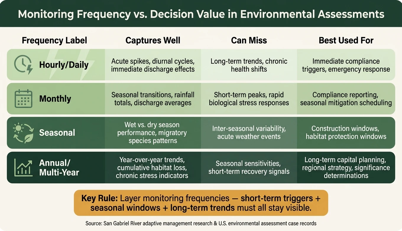
Monitoring Frequency vs. Decision Value in Environmental Assessments
The challenge is turning changing conditions into baseline evidence that can stand up in water, air, and biodiversity assessments. Spotting temporal patterns is only the start. The next step is making those patterns usable, testable, and defensible.
Sampling Design for Representative Baselines
A representative baseline has to sample across seasonal extremes, not just at one moment in time. That means including both wet and dry periods so the full annual flow pattern shows up in the record.
It also helps to pair two kinds of indicators. Fast-responding indicators, such as stem water potential in plants, react quickly to short-term stress. Longer-term indicators, such as canopy volume, show chronic stress that builds over time. Used together, they give you both an early signal and a longer-view check on ecosystem condition.
Another smart move is to co-locate new sensors with USGS stream gages or long-term weather stations. That ties short-term monitoring to a much older record and helps place new readings in historical context [3].
Sampling captures the record. Modeling turns that record into evidence.
Time-Series Analysis and Spatiotemporal Modeling
Collecting data over time is only the first step. Time-series analysis and spatiotemporal modeling help separate project effects from background variability, which is often where the hard part begins.
Methods such as Random Forest and Mixed Effects Models can sort natural stressors like rainfall and temperature from human-driven changes like wastewater discharge or land-use change [2]. In the San Gabriel River study, five years of monitoring showed that stem water potential responded more strongly than canopy volume. That result helped refine which indicators were most useful for tracking stress [2].
"Modeling can support adaptive management by providing early insight into relationships between management actions and ecological responses, allowing monitoring data to be evaluated within the initial years of program implementation." - Katie Irving and Eric D. Stein, Southern California Coastal Water Research Project [2]
Spatiotemporal tools bring location and timing into one analysis. In Northern Ontario's Ring of Fire region, Bowtie analysis and simulation modeling were used to test cumulative effects on the moose-wolf-caribou system across both space and time [1].
Short-Term Snapshots vs. Multi-Year Baselines: A Comparison
Baseline length shapes what an assessment can detect, test, and defend. Research suggests that at least 3 to 5 years of data are often needed to separate natural climate cycles from project-related impacts [2]. That timeline matters. If the record is too short, a wet year or dry year can look normal when it isn't.
The same pattern shows up in program design. Adaptive management frameworks like the Columbia Estuary Ecosystem Restoration Program took 12 years to mature [2]. That kind of time horizon gives managers room to see trends, test responses, and adjust course with more confidence.
Assessment Area | Short-Term Snapshot | Multi-Year Baseline | Decision Risk if Too Short |
|---|---|---|---|
Hydrology | Useful for acute disturbances | Captures seasonal extremes and historical variability | May normalize a wet or dry year |
Plant stress | Good for fast-responding indicators like stem water potential | Needed for longer-term indicators like canopy volume | May miss chronic stress |
Complex ecosystems | Helpful for rapid-response monitoring after disturbances | Better for cumulative effects and ecological tipping points | May blur natural variability with project effects |
In practice, baseline length should match the process being studied. Short records can work for acute disturbances. Multi-year records are better suited to chronic stress and cumulative effects. That choice feeds straight into significance testing, compliance calls, and mitigation timing.
How Temporal Data Shapes Decisions, Mitigation, and Risk
How Baseline Choice Affects Significance and Compliance
Once temporal data is on the table, baseline choice stops being a technical detail and becomes a compliance issue. The period an assessor selects can change how an impact is read. If that baseline does not reflect natural variability, project effects can blur together with background stressors like drought. When that happens, permitting risk goes up. It also skews significance calls, because decision-makers may struggle to tell whether a shift comes from the project or from conditions that were already in play.
The San Gabriel River study shows this problem in plain terms. Wet and dry baseline years were compared with a two-year dry effects period, which made it hard to separate drought stress from project effects. In that same study, a significant decline in habitat condition was defined as p < 0.1 based on paired t-tests comparing baseline to current conditions [2].
How Temporal Data Improves Mitigation Timing and Adaptive Management
Timing shapes mitigation just as much as the mitigation measure itself. Temporal data helps tie ecological stress signals to clear windows in the year, including seasonal vegetation cycles, migratory periods, and drought conditions. That gives managers something better than a static snapshot. It gives them a clock.
In the San Gabriel River adaptive management program, Stem Water Potential (SWP) measurements were taken during peak stress hours, from 12 p.m. to 3 p.m., to capture the most sensitive signal of plant water stress [2]. The goal was simple: give managers early warning so they could increase water delivery before mortality occurred.
A smart approach is to pair fast and slow indicators. Fast indicators can flag trouble early. Slow indicators help track cumulative damage over time. Without both, managers either react too late or miss the bigger pattern.
Build time-based thresholds into permits and monitoring plans. Seasonal construction windows, drought-triggered flow increases, and phased monitoring schedules are much easier to defend when they rest on multi-year temporal data instead of a single-season snapshot.
Monitoring Resolution and Decision Value: A Comparison
Monitoring frequency should match the decision at stake. Think of it like choosing the right camera setting: one frame might catch a flash event, while a long exposure shows the trend.
Monitoring Frequency | Captures Well | Can Miss | Best Used For |
|---|---|---|---|
Hourly/Daily | Acute spikes, diurnal cycles, immediate discharge effects | Long-term trends, chronic health shifts | Immediate compliance triggers, emergency response |
Monthly | Seasonal transitions, rainfall totals, discharge averages | Short-term peaks, rapid biological stress responses | Compliance reporting, seasonal mitigation scheduling |
Seasonal | Wet vs. dry season performance, migratory species patterns | Inter-seasonal variability, acute weather events | Construction windows, habitat protection windows |
Annual/Multi-Year | Year-over-year trends, cumulative habitat loss, chronic stress indicators | Seasonal sensitivities, short-term recovery signals | Long-term capital planning, regional strategy, significance determinations |
Layer monitoring frequencies so short-term triggers, seasonal windows, and long-term trends all stay visible.
Conclusion: Building Better Assessments with Time-Based Evidence
The evidence leads to a plain takeaway: longer records lead to stronger baselines and better decisions. When an assessment rests on a single snapshot, it may reflect an oddly wet spring or a drought year instead of normal conditions. That can skew significance testing, permit conditions, and mitigation timing. Multi-year baselines cut that risk because they show the full range of conditions a system moves through. Extended monitoring also brings patterns into view that shape compliance and adaptive management in direct ways. The Terzaghi Dam program, for example, needed 4 years of monitoring to refine metrics that better separate normal variation from change [2]. That timeline says a lot about ecological systems: meaningful patterns often take time to show themselves.
Time-based data also shifts how mitigation works on the ground. Early indicators such as stem water potential can warn managers before permanent ecological damage sets in [2]. But that only works when monitoring is built around the biological process being studied, not just a reporting cycle on a calendar.
For executives and public-sector leaders, the lesson is pretty straightforward: match monitoring length and resolution to the level of risk.
Avoid snapshot baselines in variable systems. Aim for at least 3–4 years of baseline data before drawing conclusions [2].
Match indicator speed to the process. Fast-responding indicators can flag acute stress early, while slower indicators track cumulative health over time.
Use modeling early to cut uncertainty. Ecological modeling can produce actionable insight within the first few years of a program and help teams focus enhanced monitoring where it is most needed [2].
FAQs
Why isn’t one site visit enough?
A single site visit rarely tells the whole story. Natural systems shift with seasons, weather, species movement, and human activity, so one snapshot can be misleading. If you want findings you can stand behind, you usually need multi-year monitoring and data sets with enough depth to test hypotheses with confidence.
Time matters for another reason too: many indicators change slowly. Some may take years before the signal is clear enough to measure, while short-term observations can miss long-range trends or older effects that are still shaping what you see on the ground.
How much baseline data is usually needed?
There is no fixed industry standard for baseline data in environmental assessments. What counts as enough depends on the project’s scale, its likely effects, and the rules that apply. In many cases, regulators want documents that are analytical, not encyclopedic.
That shifts the focus from sheer volume to data you can trust. High-quality, verified data matters more than a huge stack of information. Natural systems are messy and variable, so one season of fieldwork may not tell the whole story. For some initiatives, it can take years of monitoring to build a dataset that supports sound findings.
When should models be used with field monitoring?
Models belong in field monitoring from the start. When teams use them early, they can make better calls when conditions are uncertain and the path ahead isn’t fully clear. A good model helps point out the biggest unknowns, shows where monitoring effort should go first, and estimates what may happen when a management action is put in place.
When you pair models with monitoring data, they become even more useful. They can help teams adjust strategy as new information comes in and build a deeper view of how ecosystems change over time.
Related Blog Posts
Latest Articles
©2026

Narrative Change and Power Building: The Missing Half of Advocacy
Narrative change is the process of disrupting dominant narratives that normalize inequity and advancing new narratives from historically marginalized communities.

Funding Resilience Without Federal Grants
BRIC is unreliable and FEMA is shrinking. Here's how cities fund climate resilience with dedicated revenue, blended finance, and a coordinating authority.

The ESG Blind Spot: How AI Is Finding Risks in Companies Nobody Else Is Watching
Norway's sovereign wealth fund uses AI to screen 7,200 portfolio companies for forced labor and corruption within 24 hours. The real story is the emerging-market coverage gap that traditional ESG data vendors miss — and what it means for any company with a global supply chain.
Narrative Change and Power Building: The Missing Half of Advocacy
Narrative change is the process of disrupting dominant narratives that normalize inequity and advancing new narratives from historically marginalized communities.
Funding Resilience Without Federal Grants
BRIC is unreliable and FEMA is shrinking. Here's how cities fund climate resilience with dedicated revenue, blended finance, and a coordinating authority.
The ESG Blind Spot: How AI Is Finding Risks in Companies Nobody Else Is Watching
Norway's sovereign wealth fund uses AI to screen 7,200 portfolio companies for forced labor and corruption within 24 hours. The real story is the emerging-market coverage gap that traditional ESG data vendors miss — and what it means for any company with a global supply chain.
FAQ
01
What does it really mean to “redefine profit”?
02
What makes Council Fire different?
03
Who does Council Fire work with?
04
What does working with Council Fire actually look like?
05
How does Council Fire help organizations turn big goals into action?
06
How does Council Fire define and measure success?
07
How does technology fit into Council Fire’s work?
Jul 20, 2026
How Temporal Data Impacts Environmental Assessments
Sustainability Strategy
In This Article
Why multi-year (3–5+ years) and layered monitoring are essential for reliable environmental baselines and decisions.
How Temporal Data Impacts Environmental Assessments
A one-time site check can miss the risk. In the cases cited here, 23 people died, 167 were injured, 558 buildings were damaged, and losses went above $1 billion when hazard mapping failed to reflect a long time record instead of a fixed view.
If I had to sum up the article in one line, it’s this: time changes what an assessment says, what a permit allows, and what a team misses. Short records can make a dry year look normal, miss first-flush pollution pulses, and blur project effects with weather swings. The article points to a simple rule of thumb: use repeated monitoring across seasons and, in many cases, at least 3 to 5 years of data before making high-stakes calls.
Here’s the core takeaway in plain terms:
Daily data can show short spikes, like ash, sediment, or discharge pulses.
Seasonal data can show wet/dry shifts, plant stress windows, and species timing.
Year-to-year data can help separate project effects from drought or rainfall cycles.
Long-term data can show slow trend lines, cumulative effects, and climate-driven change.
Short baselines increase decision risk because they can misread what “normal” looks like.
Layered monitoring works best: short-interval sensors for fast events, plus multi-year records for trend testing.
Fast and slow indicators should be used together so teams can see both early stress and longer damage.
Models help early, but they work better when paired with repeated field data.
I’d frame the article this way: if you’re making U.S. planning, permitting, or compliance decisions, time is not a side detail. It is part of the evidence.
How Temporal Baselines Shape Core Assessment Findings
Hydrology, Water Quality, and Climate Signals
Timing can change the whole story an assessment tells. Temporal resolution decides whether you catch short, messy pulses in a system or smooth them out until they barely show up. A short water-monitoring window can easily miss rare spikes and make an unusually wet or dry year seem normal.
After the 2022 Hermit's Peak - Calf Canyon Fire, semi-continuous sensors were deployed within two weeks and tracked ash and sediment 190 km downstream, while local treatment failed [3]. That matters because grab sampling would have missed much of the first-flush pulse [3].
U.S. case records show the same pattern again and again: ash, sediment, wastewater, and oil do not stay put. They can travel tens to hundreds of kilometers downstream, reaching intakes, waterways, and nearby communities [3].
The timing issue does not stop with water. It shows up in ecological surveys too, where the season of a site visit can shape what the site seems to support.
Why Biodiversity Surveys Depend on Timing and Repeat Visits
Ecological conditions shift through the year, so one visit almost never defines baseline habitat quality. A spring survey and a late-summer survey can paint very different pictures of the same place. That is why repeat visits matter. They help separate normal seasonal change from effects tied to a project.
In the San Gabriel River, researchers needed 5 years of monitoring to distinguish reduced wastewater discharge from dry-year stress [2].
The point is simple: a one-season survey shows conditions at the moment of sampling, not the full range of swings a system goes through. Repeat visits across multiple seasons and years build a baseline that is easier to defend.
How Long Is a Phase I ESA Actually Good For? When Does It Expire? | Resource Management Associates
Methods for Turning Temporal Data into Usable Evidence
Monitoring Frequency vs. Decision Value in Environmental Assessments
The challenge is turning changing conditions into baseline evidence that can stand up in water, air, and biodiversity assessments. Spotting temporal patterns is only the start. The next step is making those patterns usable, testable, and defensible.
Sampling Design for Representative Baselines
A representative baseline has to sample across seasonal extremes, not just at one moment in time. That means including both wet and dry periods so the full annual flow pattern shows up in the record.
It also helps to pair two kinds of indicators. Fast-responding indicators, such as stem water potential in plants, react quickly to short-term stress. Longer-term indicators, such as canopy volume, show chronic stress that builds over time. Used together, they give you both an early signal and a longer-view check on ecosystem condition.
Another smart move is to co-locate new sensors with USGS stream gages or long-term weather stations. That ties short-term monitoring to a much older record and helps place new readings in historical context [3].
Sampling captures the record. Modeling turns that record into evidence.
Time-Series Analysis and Spatiotemporal Modeling
Collecting data over time is only the first step. Time-series analysis and spatiotemporal modeling help separate project effects from background variability, which is often where the hard part begins.
Methods such as Random Forest and Mixed Effects Models can sort natural stressors like rainfall and temperature from human-driven changes like wastewater discharge or land-use change [2]. In the San Gabriel River study, five years of monitoring showed that stem water potential responded more strongly than canopy volume. That result helped refine which indicators were most useful for tracking stress [2].
"Modeling can support adaptive management by providing early insight into relationships between management actions and ecological responses, allowing monitoring data to be evaluated within the initial years of program implementation." - Katie Irving and Eric D. Stein, Southern California Coastal Water Research Project [2]
Spatiotemporal tools bring location and timing into one analysis. In Northern Ontario's Ring of Fire region, Bowtie analysis and simulation modeling were used to test cumulative effects on the moose-wolf-caribou system across both space and time [1].
Short-Term Snapshots vs. Multi-Year Baselines: A Comparison
Baseline length shapes what an assessment can detect, test, and defend. Research suggests that at least 3 to 5 years of data are often needed to separate natural climate cycles from project-related impacts [2]. That timeline matters. If the record is too short, a wet year or dry year can look normal when it isn't.
The same pattern shows up in program design. Adaptive management frameworks like the Columbia Estuary Ecosystem Restoration Program took 12 years to mature [2]. That kind of time horizon gives managers room to see trends, test responses, and adjust course with more confidence.
Assessment Area | Short-Term Snapshot | Multi-Year Baseline | Decision Risk if Too Short |
|---|---|---|---|
Hydrology | Useful for acute disturbances | Captures seasonal extremes and historical variability | May normalize a wet or dry year |
Plant stress | Good for fast-responding indicators like stem water potential | Needed for longer-term indicators like canopy volume | May miss chronic stress |
Complex ecosystems | Helpful for rapid-response monitoring after disturbances | Better for cumulative effects and ecological tipping points | May blur natural variability with project effects |
In practice, baseline length should match the process being studied. Short records can work for acute disturbances. Multi-year records are better suited to chronic stress and cumulative effects. That choice feeds straight into significance testing, compliance calls, and mitigation timing.
How Temporal Data Shapes Decisions, Mitigation, and Risk
How Baseline Choice Affects Significance and Compliance
Once temporal data is on the table, baseline choice stops being a technical detail and becomes a compliance issue. The period an assessor selects can change how an impact is read. If that baseline does not reflect natural variability, project effects can blur together with background stressors like drought. When that happens, permitting risk goes up. It also skews significance calls, because decision-makers may struggle to tell whether a shift comes from the project or from conditions that were already in play.
The San Gabriel River study shows this problem in plain terms. Wet and dry baseline years were compared with a two-year dry effects period, which made it hard to separate drought stress from project effects. In that same study, a significant decline in habitat condition was defined as p < 0.1 based on paired t-tests comparing baseline to current conditions [2].
How Temporal Data Improves Mitigation Timing and Adaptive Management
Timing shapes mitigation just as much as the mitigation measure itself. Temporal data helps tie ecological stress signals to clear windows in the year, including seasonal vegetation cycles, migratory periods, and drought conditions. That gives managers something better than a static snapshot. It gives them a clock.
In the San Gabriel River adaptive management program, Stem Water Potential (SWP) measurements were taken during peak stress hours, from 12 p.m. to 3 p.m., to capture the most sensitive signal of plant water stress [2]. The goal was simple: give managers early warning so they could increase water delivery before mortality occurred.
A smart approach is to pair fast and slow indicators. Fast indicators can flag trouble early. Slow indicators help track cumulative damage over time. Without both, managers either react too late or miss the bigger pattern.
Build time-based thresholds into permits and monitoring plans. Seasonal construction windows, drought-triggered flow increases, and phased monitoring schedules are much easier to defend when they rest on multi-year temporal data instead of a single-season snapshot.
Monitoring Resolution and Decision Value: A Comparison
Monitoring frequency should match the decision at stake. Think of it like choosing the right camera setting: one frame might catch a flash event, while a long exposure shows the trend.
Monitoring Frequency | Captures Well | Can Miss | Best Used For |
|---|---|---|---|
Hourly/Daily | Acute spikes, diurnal cycles, immediate discharge effects | Long-term trends, chronic health shifts | Immediate compliance triggers, emergency response |
Monthly | Seasonal transitions, rainfall totals, discharge averages | Short-term peaks, rapid biological stress responses | Compliance reporting, seasonal mitigation scheduling |
Seasonal | Wet vs. dry season performance, migratory species patterns | Inter-seasonal variability, acute weather events | Construction windows, habitat protection windows |
Annual/Multi-Year | Year-over-year trends, cumulative habitat loss, chronic stress indicators | Seasonal sensitivities, short-term recovery signals | Long-term capital planning, regional strategy, significance determinations |
Layer monitoring frequencies so short-term triggers, seasonal windows, and long-term trends all stay visible.
Conclusion: Building Better Assessments with Time-Based Evidence
The evidence leads to a plain takeaway: longer records lead to stronger baselines and better decisions. When an assessment rests on a single snapshot, it may reflect an oddly wet spring or a drought year instead of normal conditions. That can skew significance testing, permit conditions, and mitigation timing. Multi-year baselines cut that risk because they show the full range of conditions a system moves through. Extended monitoring also brings patterns into view that shape compliance and adaptive management in direct ways. The Terzaghi Dam program, for example, needed 4 years of monitoring to refine metrics that better separate normal variation from change [2]. That timeline says a lot about ecological systems: meaningful patterns often take time to show themselves.
Time-based data also shifts how mitigation works on the ground. Early indicators such as stem water potential can warn managers before permanent ecological damage sets in [2]. But that only works when monitoring is built around the biological process being studied, not just a reporting cycle on a calendar.
For executives and public-sector leaders, the lesson is pretty straightforward: match monitoring length and resolution to the level of risk.
Avoid snapshot baselines in variable systems. Aim for at least 3–4 years of baseline data before drawing conclusions [2].
Match indicator speed to the process. Fast-responding indicators can flag acute stress early, while slower indicators track cumulative health over time.
Use modeling early to cut uncertainty. Ecological modeling can produce actionable insight within the first few years of a program and help teams focus enhanced monitoring where it is most needed [2].
FAQs
Why isn’t one site visit enough?
A single site visit rarely tells the whole story. Natural systems shift with seasons, weather, species movement, and human activity, so one snapshot can be misleading. If you want findings you can stand behind, you usually need multi-year monitoring and data sets with enough depth to test hypotheses with confidence.
Time matters for another reason too: many indicators change slowly. Some may take years before the signal is clear enough to measure, while short-term observations can miss long-range trends or older effects that are still shaping what you see on the ground.
How much baseline data is usually needed?
There is no fixed industry standard for baseline data in environmental assessments. What counts as enough depends on the project’s scale, its likely effects, and the rules that apply. In many cases, regulators want documents that are analytical, not encyclopedic.
That shifts the focus from sheer volume to data you can trust. High-quality, verified data matters more than a huge stack of information. Natural systems are messy and variable, so one season of fieldwork may not tell the whole story. For some initiatives, it can take years of monitoring to build a dataset that supports sound findings.
When should models be used with field monitoring?
Models belong in field monitoring from the start. When teams use them early, they can make better calls when conditions are uncertain and the path ahead isn’t fully clear. A good model helps point out the biggest unknowns, shows where monitoring effort should go first, and estimates what may happen when a management action is put in place.
When you pair models with monitoring data, they become even more useful. They can help teams adjust strategy as new information comes in and build a deeper view of how ecosystems change over time.
Related Blog Posts
Latest Articles
©2026
Narrative Change and Power Building: The Missing Half of Advocacy
Narrative change is the process of disrupting dominant narratives that normalize inequity and advancing new narratives from historically marginalized communities.
Funding Resilience Without Federal Grants
BRIC is unreliable and FEMA is shrinking. Here's how cities fund climate resilience with dedicated revenue, blended finance, and a coordinating authority.
The ESG Blind Spot: How AI Is Finding Risks in Companies Nobody Else Is Watching
Norway's sovereign wealth fund uses AI to screen 7,200 portfolio companies for forced labor and corruption within 24 hours. The real story is the emerging-market coverage gap that traditional ESG data vendors miss — and what it means for any company with a global supply chain.
FAQ
01
What does it really mean to “redefine profit”?
02
What makes Council Fire different?
03
Who does Council Fire work with?
04
What does working with Council Fire actually look like?
05
How does Council Fire help organizations turn big goals into action?
06
How does Council Fire define and measure success?
07
How does technology fit into Council Fire’s work?
Jul 20, 2026
How Temporal Data Impacts Environmental Assessments
Sustainability Strategy
In This Article
Why multi-year (3–5+ years) and layered monitoring are essential for reliable environmental baselines and decisions.
How Temporal Data Impacts Environmental Assessments
A one-time site check can miss the risk. In the cases cited here, 23 people died, 167 were injured, 558 buildings were damaged, and losses went above $1 billion when hazard mapping failed to reflect a long time record instead of a fixed view.
If I had to sum up the article in one line, it’s this: time changes what an assessment says, what a permit allows, and what a team misses. Short records can make a dry year look normal, miss first-flush pollution pulses, and blur project effects with weather swings. The article points to a simple rule of thumb: use repeated monitoring across seasons and, in many cases, at least 3 to 5 years of data before making high-stakes calls.
Here’s the core takeaway in plain terms:
Daily data can show short spikes, like ash, sediment, or discharge pulses.
Seasonal data can show wet/dry shifts, plant stress windows, and species timing.
Year-to-year data can help separate project effects from drought or rainfall cycles.
Long-term data can show slow trend lines, cumulative effects, and climate-driven change.
Short baselines increase decision risk because they can misread what “normal” looks like.
Layered monitoring works best: short-interval sensors for fast events, plus multi-year records for trend testing.
Fast and slow indicators should be used together so teams can see both early stress and longer damage.
Models help early, but they work better when paired with repeated field data.
I’d frame the article this way: if you’re making U.S. planning, permitting, or compliance decisions, time is not a side detail. It is part of the evidence.
How Temporal Baselines Shape Core Assessment Findings
Hydrology, Water Quality, and Climate Signals
Timing can change the whole story an assessment tells. Temporal resolution decides whether you catch short, messy pulses in a system or smooth them out until they barely show up. A short water-monitoring window can easily miss rare spikes and make an unusually wet or dry year seem normal.
After the 2022 Hermit's Peak - Calf Canyon Fire, semi-continuous sensors were deployed within two weeks and tracked ash and sediment 190 km downstream, while local treatment failed [3]. That matters because grab sampling would have missed much of the first-flush pulse [3].
U.S. case records show the same pattern again and again: ash, sediment, wastewater, and oil do not stay put. They can travel tens to hundreds of kilometers downstream, reaching intakes, waterways, and nearby communities [3].
The timing issue does not stop with water. It shows up in ecological surveys too, where the season of a site visit can shape what the site seems to support.
Why Biodiversity Surveys Depend on Timing and Repeat Visits
Ecological conditions shift through the year, so one visit almost never defines baseline habitat quality. A spring survey and a late-summer survey can paint very different pictures of the same place. That is why repeat visits matter. They help separate normal seasonal change from effects tied to a project.
In the San Gabriel River, researchers needed 5 years of monitoring to distinguish reduced wastewater discharge from dry-year stress [2].
The point is simple: a one-season survey shows conditions at the moment of sampling, not the full range of swings a system goes through. Repeat visits across multiple seasons and years build a baseline that is easier to defend.
How Long Is a Phase I ESA Actually Good For? When Does It Expire? | Resource Management Associates
Methods for Turning Temporal Data into Usable Evidence
Monitoring Frequency vs. Decision Value in Environmental Assessments
The challenge is turning changing conditions into baseline evidence that can stand up in water, air, and biodiversity assessments. Spotting temporal patterns is only the start. The next step is making those patterns usable, testable, and defensible.
Sampling Design for Representative Baselines
A representative baseline has to sample across seasonal extremes, not just at one moment in time. That means including both wet and dry periods so the full annual flow pattern shows up in the record.
It also helps to pair two kinds of indicators. Fast-responding indicators, such as stem water potential in plants, react quickly to short-term stress. Longer-term indicators, such as canopy volume, show chronic stress that builds over time. Used together, they give you both an early signal and a longer-view check on ecosystem condition.
Another smart move is to co-locate new sensors with USGS stream gages or long-term weather stations. That ties short-term monitoring to a much older record and helps place new readings in historical context [3].
Sampling captures the record. Modeling turns that record into evidence.
Time-Series Analysis and Spatiotemporal Modeling
Collecting data over time is only the first step. Time-series analysis and spatiotemporal modeling help separate project effects from background variability, which is often where the hard part begins.
Methods such as Random Forest and Mixed Effects Models can sort natural stressors like rainfall and temperature from human-driven changes like wastewater discharge or land-use change [2]. In the San Gabriel River study, five years of monitoring showed that stem water potential responded more strongly than canopy volume. That result helped refine which indicators were most useful for tracking stress [2].
"Modeling can support adaptive management by providing early insight into relationships between management actions and ecological responses, allowing monitoring data to be evaluated within the initial years of program implementation." - Katie Irving and Eric D. Stein, Southern California Coastal Water Research Project [2]
Spatiotemporal tools bring location and timing into one analysis. In Northern Ontario's Ring of Fire region, Bowtie analysis and simulation modeling were used to test cumulative effects on the moose-wolf-caribou system across both space and time [1].
Short-Term Snapshots vs. Multi-Year Baselines: A Comparison
Baseline length shapes what an assessment can detect, test, and defend. Research suggests that at least 3 to 5 years of data are often needed to separate natural climate cycles from project-related impacts [2]. That timeline matters. If the record is too short, a wet year or dry year can look normal when it isn't.
The same pattern shows up in program design. Adaptive management frameworks like the Columbia Estuary Ecosystem Restoration Program took 12 years to mature [2]. That kind of time horizon gives managers room to see trends, test responses, and adjust course with more confidence.
Assessment Area | Short-Term Snapshot | Multi-Year Baseline | Decision Risk if Too Short |
|---|---|---|---|
Hydrology | Useful for acute disturbances | Captures seasonal extremes and historical variability | May normalize a wet or dry year |
Plant stress | Good for fast-responding indicators like stem water potential | Needed for longer-term indicators like canopy volume | May miss chronic stress |
Complex ecosystems | Helpful for rapid-response monitoring after disturbances | Better for cumulative effects and ecological tipping points | May blur natural variability with project effects |
In practice, baseline length should match the process being studied. Short records can work for acute disturbances. Multi-year records are better suited to chronic stress and cumulative effects. That choice feeds straight into significance testing, compliance calls, and mitigation timing.
How Temporal Data Shapes Decisions, Mitigation, and Risk
How Baseline Choice Affects Significance and Compliance
Once temporal data is on the table, baseline choice stops being a technical detail and becomes a compliance issue. The period an assessor selects can change how an impact is read. If that baseline does not reflect natural variability, project effects can blur together with background stressors like drought. When that happens, permitting risk goes up. It also skews significance calls, because decision-makers may struggle to tell whether a shift comes from the project or from conditions that were already in play.
The San Gabriel River study shows this problem in plain terms. Wet and dry baseline years were compared with a two-year dry effects period, which made it hard to separate drought stress from project effects. In that same study, a significant decline in habitat condition was defined as p < 0.1 based on paired t-tests comparing baseline to current conditions [2].
How Temporal Data Improves Mitigation Timing and Adaptive Management
Timing shapes mitigation just as much as the mitigation measure itself. Temporal data helps tie ecological stress signals to clear windows in the year, including seasonal vegetation cycles, migratory periods, and drought conditions. That gives managers something better than a static snapshot. It gives them a clock.
In the San Gabriel River adaptive management program, Stem Water Potential (SWP) measurements were taken during peak stress hours, from 12 p.m. to 3 p.m., to capture the most sensitive signal of plant water stress [2]. The goal was simple: give managers early warning so they could increase water delivery before mortality occurred.
A smart approach is to pair fast and slow indicators. Fast indicators can flag trouble early. Slow indicators help track cumulative damage over time. Without both, managers either react too late or miss the bigger pattern.
Build time-based thresholds into permits and monitoring plans. Seasonal construction windows, drought-triggered flow increases, and phased monitoring schedules are much easier to defend when they rest on multi-year temporal data instead of a single-season snapshot.
Monitoring Resolution and Decision Value: A Comparison
Monitoring frequency should match the decision at stake. Think of it like choosing the right camera setting: one frame might catch a flash event, while a long exposure shows the trend.
Monitoring Frequency | Captures Well | Can Miss | Best Used For |
|---|---|---|---|
Hourly/Daily | Acute spikes, diurnal cycles, immediate discharge effects | Long-term trends, chronic health shifts | Immediate compliance triggers, emergency response |
Monthly | Seasonal transitions, rainfall totals, discharge averages | Short-term peaks, rapid biological stress responses | Compliance reporting, seasonal mitigation scheduling |
Seasonal | Wet vs. dry season performance, migratory species patterns | Inter-seasonal variability, acute weather events | Construction windows, habitat protection windows |
Annual/Multi-Year | Year-over-year trends, cumulative habitat loss, chronic stress indicators | Seasonal sensitivities, short-term recovery signals | Long-term capital planning, regional strategy, significance determinations |
Layer monitoring frequencies so short-term triggers, seasonal windows, and long-term trends all stay visible.
Conclusion: Building Better Assessments with Time-Based Evidence
The evidence leads to a plain takeaway: longer records lead to stronger baselines and better decisions. When an assessment rests on a single snapshot, it may reflect an oddly wet spring or a drought year instead of normal conditions. That can skew significance testing, permit conditions, and mitigation timing. Multi-year baselines cut that risk because they show the full range of conditions a system moves through. Extended monitoring also brings patterns into view that shape compliance and adaptive management in direct ways. The Terzaghi Dam program, for example, needed 4 years of monitoring to refine metrics that better separate normal variation from change [2]. That timeline says a lot about ecological systems: meaningful patterns often take time to show themselves.
Time-based data also shifts how mitigation works on the ground. Early indicators such as stem water potential can warn managers before permanent ecological damage sets in [2]. But that only works when monitoring is built around the biological process being studied, not just a reporting cycle on a calendar.
For executives and public-sector leaders, the lesson is pretty straightforward: match monitoring length and resolution to the level of risk.
Avoid snapshot baselines in variable systems. Aim for at least 3–4 years of baseline data before drawing conclusions [2].
Match indicator speed to the process. Fast-responding indicators can flag acute stress early, while slower indicators track cumulative health over time.
Use modeling early to cut uncertainty. Ecological modeling can produce actionable insight within the first few years of a program and help teams focus enhanced monitoring where it is most needed [2].
FAQs
Why isn’t one site visit enough?
A single site visit rarely tells the whole story. Natural systems shift with seasons, weather, species movement, and human activity, so one snapshot can be misleading. If you want findings you can stand behind, you usually need multi-year monitoring and data sets with enough depth to test hypotheses with confidence.
Time matters for another reason too: many indicators change slowly. Some may take years before the signal is clear enough to measure, while short-term observations can miss long-range trends or older effects that are still shaping what you see on the ground.
How much baseline data is usually needed?
There is no fixed industry standard for baseline data in environmental assessments. What counts as enough depends on the project’s scale, its likely effects, and the rules that apply. In many cases, regulators want documents that are analytical, not encyclopedic.
That shifts the focus from sheer volume to data you can trust. High-quality, verified data matters more than a huge stack of information. Natural systems are messy and variable, so one season of fieldwork may not tell the whole story. For some initiatives, it can take years of monitoring to build a dataset that supports sound findings.
When should models be used with field monitoring?
Models belong in field monitoring from the start. When teams use them early, they can make better calls when conditions are uncertain and the path ahead isn’t fully clear. A good model helps point out the biggest unknowns, shows where monitoring effort should go first, and estimates what may happen when a management action is put in place.
When you pair models with monitoring data, they become even more useful. They can help teams adjust strategy as new information comes in and build a deeper view of how ecosystems change over time.
Related Blog Posts
Latest Articles
©2026
Narrative Change and Power Building: The Missing Half of Advocacy
Narrative change is the process of disrupting dominant narratives that normalize inequity and advancing new narratives from historically marginalized communities.
Funding Resilience Without Federal Grants
BRIC is unreliable and FEMA is shrinking. Here's how cities fund climate resilience with dedicated revenue, blended finance, and a coordinating authority.
The ESG Blind Spot: How AI Is Finding Risks in Companies Nobody Else Is Watching
Norway's sovereign wealth fund uses AI to screen 7,200 portfolio companies for forced labor and corruption within 24 hours. The real story is the emerging-market coverage gap that traditional ESG data vendors miss — and what it means for any company with a global supply chain.
FAQ
What does it really mean to “redefine profit”?
What makes Council Fire different?
Who does Council Fire work with?
What does working with Council Fire actually look like?
How does Council Fire help organizations turn big goals into action?
How does Council Fire define and measure success?
How does technology fit into Council Fire’s work?