In This Article
Assess project contributions amid data gaps by comparing with/without scenarios, reporting ranges, and tying findings to owners.
Cumulative Impacts: Project Uncertainty and Data Gaps
We can assess a project’s contribution without perfect data - but we must show where the estimate could change. We compare matched futures with and without the project, report ranges, and identify missing information that could change the decision.
Context matters. In the article’s fictional watershed example, the same 0.50 million gallons per day withdrawal leaves ample water in one case but pushes flow below a threshold in another. The project’s share alone does not tell us whether harm could occur.
We build the assessment around five steps:
Set the scope: Identify affected people and resources, boundaries, time periods, and other actions.
Check the baseline: Separate measured conditions from forecasts and prioritize gaps that could change the choice.
Compare plausible futures: Keep nonproject assumptions matched and distinguish uncertainty from actual differences across seasons or locations.
Test the findings: Check assumptions, thresholds, mitigation, and effects that remain after controls.
Record the next step: Proceed with controls, revise the project, gather data, or defer the conclusion.
Our rule is simple: <u>missing data do not mean no impact</u>. We connect each finding to a clear limit, a responsible party, and a trigger for review.
Set Assessment Boundaries and Establish the Baseline
Identify Receptors, Boundaries, and Other Actions
Set the scope before choosing methods. Map each receptor - people, drinking-water sources, wetlands, wildlife, or cultural resources - to the stressors and exposure pathways that affect it. Draw boundaries around functional areas, such as watersheds, airsheds, aquifers, corridors, or cultural landscapes, rather than property lines. Include private wells, subsistence activities, and communities that may bear disproportionate burdens. Area averages can hide concentrated exposure. For each receptor, record the boundary, exposure metric, time window, and reasoning.[5][6][11]
Maintain an action register that carries existing, approved, foreseeable, and potential actions into scenario development.
| Scope element | Geographic scale | Time period | Confidence and scope assumptions |
|---|---|---|---|
| Receptor boundary | Relevant watershed, airshed, habitat, aquifer, or community area | Full exposure period | Explain pathway evidence and identify poorly monitored areas |
| Historical conditions | Area with legacy pressures | Available trend record | Note inconsistent records and major land-use changes |
| Project phases | Construction footprint and connected exposure areas | Construction, operation, closure, and post-closure | Record schedules, operating conditions, and lasting effects |
| Existing actions | Sources affecting the same receptors | Current operations and expected remaining life | Verify activity and identify pressures already included in baseline data |
| Approved actions | Overlapping exposure areas | Expected construction and operation | Approval does not mean implementation; verify funding and construction status |
| Foreseeable actions | Areas connected to shared receptors | Documented planning horizon | Cite applications, contracts, plans, or agency commitments |
| Potential future actions | Areas where added development could matter | Uncertain timing | Test separately in sensitivity analysis; do not treat as expected development |
Describe Baseline Trends and Data Quality
Build a baseline timeline that tracks observations, disturbances, land-use changes, and monitoring gaps. Keep observed conditions separate from the future without the project. That future must account for likely changes in climate, regulations, maintenance, abandonment, and development. Count each existing pressure only once.[8][9]
| Evidence source | Strength and appropriate use | Main limit | Confidence |
|---|---|---|---|
| Regulatory or facility monitoring | Measured concentrations and operating history | May miss events, pollutants, or off-site locations | Depends on coverage, calibration, and quality controls |
| Independent studies | Trends and receptor-response relationships | Methods and study populations may differ | Depends on study design and local relevance |
| Remote sensing | Land-cover change, heat, and vegetation patterns | Resolution and indirect indicators limit exposure estimates | Depends on scale and validation |
| Field surveys | Direct habitat, species, and exposure information | Seasonal access and detection limits | Depends on sampling design and timing |
| Community knowledge | Historical changes, uses, and missed events | Collection and interpretation require agreed procedures | Assess documentation and supporting evidence |
| Indigenous knowledge | Long-term ecological and cultural understanding | Requires consent, confidentiality, and knowledge governance | Determine collaboratively; do not reduce to a numerical score |
| Models | Spatial gaps and future conditions | Results depend on inputs and assumptions | Report validation and uncertainty |
For each dataset, record its date, coverage, frequency, method, detection limits, missing values, quality control, calibration, metadata, and known bias. Label conditions as measured, modeled, inferred, or judgment-based. Use consistent U.S. units and averaging periods, and distinguish annual averages from seasonal or event-based measurements.[2][7] This documentation defines the baseline for comparing scenarios.
Prioritize Data Gaps That Could Change the Decision
Rank gaps by their effect on the decision, not by how easy the data are to collect. Focus on missing exposure data, seasonal extremes, stressor estimates, or receptor-response relationships that could change a significance finding, mitigation requirement, alternative selection, or protected-receptor assessment. Match the gap to targeted sampling, seasonal monitoring, modeling, or expert review. Record who will address it, the deadline, and which decision remains conditional if the gap is not resolved.[2][6]
Before transferring data from another location, compare climate, geology, hydrology, source mix, receptor sensitivity, methods, and timing. Regional monitoring may support background estimates without representing fence-line exposure. Label transferred values as estimates, explain the differences, and carry those limits into contribution ranges. Keep poorly monitored areas within scientifically justified boundaries: missing data do not demonstrate no impact.[6][9]
Use the documented boundaries, trends, and gaps to build with-project and without-project scenarios.
sbb-itb-8baf5f1
Addressing cumulative effects & risk and uncertainty in marine decision-making
Build Scenarios and Estimate Project Contributions
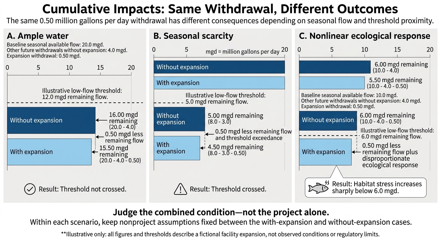
Cumulative Impacts: Same Withdrawal, Different Outcomes
Define Plausible Development Scenarios
Build scenarios around documented uncertainty and data gaps, not growth projections alone. Scenarios test plausible futures; they are not predictions. Pair every with-project case with a without-project case, keeping nonproject conditions the same.
Use the matrix below to specify included and excluded actions, geographic and time boundaries, operating assumptions, data sources, implementation likelihood, and revision triggers. Assign probabilities only when permits, funding, schedules, commitments, completion history, or a defensible forecast support them.[3] Use the baseline and data-gap inventory to set each scenario’s bounds.
| Scenario and purpose | Included / excluded actions | Timing and operations | Sources and implementation likelihood | Revision trigger / decision use |
|---|---|---|---|---|
| Current trend: reference case | Existing activities and documented trends; exclude separate future-project additions | Continue documented operating patterns over the assessment horizon | Monitoring and trend records; confidence depends on trend stability | Updated observations or reference comparison |
| Committed development: test supported additions | Funded, approved, or advancing actions; exclude unsupported proposals | Use documented startup dates and capacity | Permits, funding, construction records; distinguish approval from likely implementation | Funding or schedule change / operating conditions |
| Reasonably foreseeable development: test plausible growth | Evidence-backed proposals beyond committed actions; exclude remote possibilities | Test supported timing and operating ranges | Applications, plans, commitments; state remaining uncertainty | Permit or capacity change / mitigation needs |
| Stress test: identify vulnerabilities | Adverse but plausible combinations; exclude physically inconsistent extremes | Align drought, peak demand, and overlapping operations | Flow records and engineering limits; not an expected outcome | New hazard evidence / resilience measures |
| Alternative design/timing: compare options | Change project design, controls, or schedule; retain the same nonproject actions | Test phasing, seasonal limits, or reduced demand | Design specifications; benefits depend on implementation | Design revision / alternative selection |
Count each action once across scenarios. Choose the simplest method that fits the data and the decision.
Choose Methods and Report Contribution Ranges
Match the method to the effect: additive accounting for independent effects, interaction or threshold analysis for nonlinear effects, trend analysis for baseline trajectories, exposure overlays for spatial receptors, and scenario modeling for future conditions.
Let data quality guide the analysis. Use measurements where available, models to address gaps, and ranges for uncertain inputs. When numbers would mislead, use qualitative judgment and document its evidence and confidence.
Report each component separately: existing conditions, project-only effects, other-action contributions, combined conditions, the incremental difference, and residual effects after mitigation. Do not merge unlike indicators - such as acres of habitat, pounds of emissions, and health-risk probabilities - into one score unless you explicitly justify the aggregation method and value judgments.[1][2]
| Measure | Example use | Main limit |
|---|---|---|
| Absolute change | An added 2.0 million gallons per day of withdrawal | May not show relative importance in a large system |
| Percentage contribution | Project contributes 8% of total modeled annual load | Denominator must be defined; a small share can still be harmful |
| Affected area | An additional 12 acres of seasonal wetland exposure | Spatial aggregation can hide concentrated effects |
| Duration | Exposure occurs for 6 months per year for 10 years | Short duration may still coincide with a sensitive life stage |
| Frequency | Threshold exceedance occurs 4 days per summer | Average conditions can conceal episodic events |
| Intensity | Peak concentration rises by 5 micrograms per liter | Peak and average effects can lead to different conclusions |
| Threshold or risk status | Combined condition crosses a water-quality or health benchmark | Thresholds may be uncertain, nonlinear, or protective rather than predictive |
State the denominator for every percentage. Explain why even a small share can matter near a threshold or during a critical season. Label each range as uncertainty, variability, or scenario range. Keep correlated inputs together - for example, drought, low flow, and higher demand - rather than combining unrelated extremes.
Check whether the project adds stress, brings threshold crossings forward, shifts exposure, or increases risk. Identify mitigation assumptions and unresolved gaps that could change the decision.[1][2][3]
The example below shows how the same project contribution can be negligible in one setting and cross a threshold in another.
Hypothetical Example: Facility Expansion in a Shared Watershed
Illustrative only: All figures, units, and thresholds below describe a fictional facility expansion, not observed conditions or regulatory limits. In each row, nonproject assumptions remain fixed.[4]
Scenario Baseline seasonal available flow Other future withdrawals without expansion Expansion withdrawal Illustrative low-flow threshold Result with expansion Incremental effect A: Ample water 20.0 mgd 4.0 mgd 0.50 mgd 12.0 mgd remaining flow 15.50 mgd remains; threshold not crossed 0.50 mgd less remaining flow B: Seasonal scarcity 8.0 mgd 3.0 mgd 0.50 mgd 5.0 mgd remaining flow 4.50 mgd remains; threshold crossed 0.50 mgd less remaining flow and threshold exceedance C: Nonlinear ecological response 10.0 mgd 4.0 mgd 0.50 mgd 6.0 mgd remaining flow 5.50 mgd remains; habitat stress increases sharply below 6.0 mgd 0.50 mgd less remaining flow plus disproportionate ecological response Depending on seasonal flow and threshold proximity, the same withdrawal can shift from potentially acceptable to significant, changing mitigation or operating requirements.
Report units, time period, baseline definition, threshold source, and averaging basis.[4]
Test Assumptions and State the Limits
Use the scenario ranges and data-gap inventory from the previous section to check whether the conclusion still holds.
Classify Uncertainty and Test Key Assumptions
Maintain an assumption register that covers data quality, model parameters and structure, future development, implementation, mitigation performance, and receptor response. Separate uncertainty from variability. For each assumption, record its source, date, rationale, plausible range, responsible reviewer, consequence if wrong, and review trigger. Give priority to assumptions that could change significance, the preferred alternative, vulnerable receptors, or the direction of the conclusion.[1][2]
Test influential inputs both separately and together. Include baseline trends, model structure, receptor responses, and mitigation performance. A finding holds up when its direction and decision category remain unchanged across plausible changes. Label findings that shift with small adjustments as decision-sensitive. Scenario ranges are not statistical confidence intervals; keep them separate.[13][2]
Use Cautious Assumptions and Set Analysis Limits
Use conservative assumptions tailored to each receptor when underestimating harm could matter and the direction of uncertainty is known. Explain how those assumptions protect the receptor. If new data could change the decision, collect it. Otherwise, restrict the conclusion to the conditions tested.
Do not combine incompatible datasets, count uncommitted projects as committed actions, or assume mitigation eliminates all effects without estimating residual impacts. Reconcile and disclose differences in definitions, spatial scales, time periods, detection limits, or data quality. State the model’s valid range and identify claims it cannot support.[10]
Judge the combined condition - not the project alone against receptor-specific thresholds, planning benchmarks, and enforceable limits. Keep these categories distinct:
Scientific thresholds link to receptor responses.
Planning benchmarks support screening or management.
Enforceable limits come from applicable requirements.
For each comparison, identify the authority, purpose, averaging period, and affected receptor. Verify current federal, state, Tribal, and local requirements for the action and jurisdiction. No single U.S. cumulative-impact standard applies to every assessment. Being below a legal limit does not establish that combined effects are harmless.[12][2]
Check Conclusions Against the Evidence
Use a quality-control table for each major conclusion about the project’s contribution. Record sources, tests, assumptions, and competing explanations. State whether the evidence comes from direct observations, modeling, or expert judgment, and seek independent review for high-stakes judgments. When magnitude or causation has not been established, use a directional, qualitative, or unresolved conclusion rather than an unsupported number.[1][2]
| Conclusion | Evidence and assumptions | Uncertainty and confidence | Tests and decision limits |
|---|---|---|---|
| Stable quantitative | Record measurements, the validated model, receptor, assessment period, and required assumptions | Identify remaining data or parameter uncertainty and explain confidence | Record tested ranges and residual impacts; restrict the claim to tested conditions |
| Conditional | Record supporting evidence and the assumption on which the claim depends | Identify scenario, implementation, or mitigation uncertainty | State what would reverse the conclusion and what data or project change is needed |
| Directional or qualitative conclusion | Record evidence for the direction or mechanism, without claiming a reliable magnitude | Explain gaps in exposure data, model structure, or receptor responses | Avoid a precise effect estimate; specify the study needed |
| Unresolved | Record conflicting evidence or missing decision-critical information | Explain why confidence is insufficient | State what cannot be decided and the trigger for reassessment |
Uncertainty checklist
[ ] Register sources, ranges, owners, and triggers; distinguish uncertainty, variability, scenarios, and statistical intervals.
[ ] Test influential inputs, interactions, model structures, and mitigation.
[ ] Reconcile datasets or disclose conflicts.
[ ] Justify cautious assumptions and confidence ratings.
[ ] Verify benchmark authority and applicable requirements.
[ ] Record residual impacts, unresolved claims, decision-changing data, and monitoring triggers.[1][2][13]
Carry forward only the surviving assumptions, limits, and unresolved gaps into the decision record and monitoring plan.
Conclusion: Record Decisions and Next Steps
After testing uncertainty, document the decision path and the conditions supporting it. A sound decision connects boundaries, baseline evidence, scenarios, and contribution ranges to a clear next step. Show whether remaining uncertainty could change the choice. Uncertainty does not end the assessment - it changes what you must document, monitor, or defer.
Connect Findings to Mitigation and Monitoring
Turn each material contribution into a commitment: avoidance, design changes, construction phasing, operating limits, or contingency measures. Identify the responsible party, deadline, expected effect, and verification method. Distinguish project-owned measures from shared responsibilities, and explain what happens if another party fails to deliver.
Monitor decision-critical assumptions, controls, and control performance. Define indicators, locations, methods, frequency, quality controls, data owners, reporting deadlines, triggers, corrective responses, and review authority.[15][16] Classify gaps as resolve before decision, resolve before construction, or monitor during implementation. Monitoring cannot replace evidence required before an irreversible or high-consequence decision.
Complete the Decision Record
Use the template below to keep the final record in one place. Update it when monitoring results or new development change the conditions supporting the assessment.
| Record field | Information to enter |
|---|---|
| Decision and scope | Proposed action, alternatives, authority, receptors, boundaries, time horizon, and exclusions |
| Baseline | Conditions, trends, sources, methods, last update, and data-quality limits |
| Other actions and stressors | Existing, approved, and reasonably foreseeable actions considered |
| Data gaps | Missing information, importance, affected receptor, resolution deadline, and remedy |
| Scenarios | Key assumptions and reasons each scenario is plausible |
| Contribution estimates | Project-only and cumulative results, units, locations, periods, central estimates, ranges, and confidence |
| Assumptions and limits | Model and attribution limits, thresholds, unmodeled interactions, and conditions that invalidate conclusions |
| Mitigation | Mitigation measures, owners, schedules, and enforceability |
| Residual impacts | Remaining effects, affected receptors, burden distribution, and significance by scenario |
| Monitoring and triggers | Indicators, locations, frequency, methods, owner, reporting schedule, triggers, corrective actions, and authority |
| Unresolved issues and review | Open questions, follow-up, decision conditions, and review date: Nov. 7, 2026 |
| Decision path | Selected path and supporting rationale |
Document one path: proceed with controls when evidence shows effects can be managed; revise the project when design or timing changes can reduce its contribution; gather evidence to inform the decision when a targeted study could resolve the choice; or defer a conclusion when potentially significant or irreversible effects remain unresolved. Tie the selected path directly to the evidence.[2][14]
FAQs
How do we know when data gaps are too significant to proceed?
Data gaps are too large when they prevent well-supported decisions or could hide project impacts. Before finalizing findings, document key gaps and explain how they affect decision-making.
Address these gaps with pathway-specific measurements, secondary sources, or proxies. Prioritize data quality over quantity. When the data cannot support high-stakes decisions, monitor over multiple years to separate project impacts from natural variability. For acute threats, put needed protections in place immediately while the investigation continues.
How should we weigh conflicting scenario results?
Use at least three or four scenarios to test a range of outcomes: a moderate-change baseline, adverse cases, and compound cases that combine stressors. Compare how each project or asset performs across these scenarios. Give priority to options that hold up under several conditions - not just when every assumption goes right.
For each chart or model, explain what changed, why it matters, and how management plans to respond. Link the results to clear actions so readers can see how the analysis guides decisions.
What if several small projects jointly cross an impact threshold?
Treat a combined threshold exceedance as a cumulative-risk trigger - not proof of attribution. Use predefined decision rules and baseline/reference comparisons, preferably a before-after-control-impact (BACI) design, to check whether changes fall outside seasonal or reference ranges.
Document uncertainty and other possible drivers. Keep flagged observations, verify measurement quality and detection limits, and confirm pathways and timing across projects. If the data can’t separate background effects from those layered on by projects, expand monitoring rather than force attribution.



FAQ