Sep 25, 2026 · 20 min read
Sustainability Strategy
In This Article
Time is part of biodiversity data: align surveys to species biology, standardize repeats, separate data layers, and set action thresholds.
On this page
- 1. Design a baseline that covers the right seasons and years
- Lecture 38: EIA Methods for Ecology (Baseline Study)
- 2. Standardize repeat surveys and choose indicators that show real change
- 3. Manage and compare data for time-series analysis
- 4. Apply temporal data in impact reports and project decisions
- Conclusion: Core rules for defensible temporal biodiversity data
- FAQs
Good Practices for Temporal Biodiversity Data
One site visit is often not enough. If you survey at the wrong time, you can miss breeding, migration, flowering, spawning, or seasonal water patterns - and that can lead to the wrong call in impact review.
I’d boil the article down to this: match survey timing to biology, keep repeat surveys consistent, manage the data in separate layers, and tie results to clear thresholds and actions. For higher-risk projects, that often means multi-season work and, in some cases, at least one full year of baseline data. The article also stresses that non-detection is not absence, and that comparisons only work when season, effort, method, location, and taxonomy line up.
Here’s the plain-English takeaway:
Plan surveys around impact pathways such as clearing, noise, lighting, drainage change, traffic, and water use.
Time fieldwork to species activity like breeding windows, migration periods, wet-weather amphibian calls, and plant flowering.
Repeat surveys the same way each time so changes in results are less likely to come from drift in method.
Record field conditions such as wind, rain, water level, visibility, and temperature, because they can change detection rates.
Keep raw, cleaned, analysis, and reported data separate so every result can be traced back.
Compare like with like across years; a spring survey should not be judged against a fall survey as if they mean the same thing.
Set thresholds before results come in so monitoring leads to action, not debate after the fact.
What I like about the piece is that it stays focused on decisions. It is not just about collecting more data. It is about collecting the right data, at the right times, and using them in a way that can support permitting, mitigation, monitoring, and project changes when needed.
In short, the article makes one point very clearly: time is part of the data. If timing is off, the baseline can be off too.
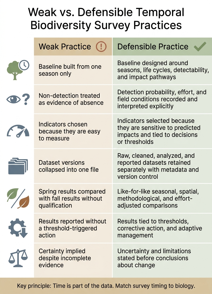
Weak vs. Defensible Temporal Biodiversity Survey Practices
1. Design a baseline that covers the right seasons and years
Start with impact pathways and priority biodiversity values
Start with a simple question: what could this project affect? Then set survey dates around that answer.
The baseline should support decisions, not just fill a file. That means focusing on which species, habitats, or ecological functions could be disturbed, during which project phases, and at what point those effects would trigger avoidance, mitigation, redesign, or monitoring.
Map each likely disturbance pathway - vegetation clearing, noise, altered drainage, lighting, dust, traffic, collision risk, or operational disturbance - to the biodiversity values exposed to it. That step gives the baseline its shape. A solar facility, for instance, creates one set of survey priorities for grassland birds and pollinators. A transmission line crossing a riparian corridor creates another. Once that map is in place, you can see which species and habitats need surveys, where those surveys belong, and when they need to happen.
Use the same logic to set the geographic scope. Start at the project footprint, then move outward through each impact pathway to include connected habitats, movement corridors, and upstream or downstream areas - not just the construction boundary. This helps align the survey period with the full zone of influence. For a wetland-dependent amphibian, that may mean adjacent uplands. For a wide-ranging raptor, it may mean a much larger foraging area.
Use a seasonal risk matrix to set survey timing
Once the priority values are clear, build a simple matrix with biodiversity values in the rows and months or biologically relevant seasons in the columns. For each cell, assess detectability, biological importance, and overlap with project disturbance windows. Put the most weight on periods when detectability and impact risk are both high. Then add visits during biologically sensitive periods, even when detectability drops.
Breeding timing can shift by as much as four weeks between years, so fixed calendar dates are a weak guide to the right survey window. [5][6] Local conditions matter just as much. Amphibians need warm, wet nights. Bats are most active in warmer months. Marsh birds call most reliably at dawn during the breeding season. Record temperature, precipitation, wind, cloud cover, water level, and visibility during every visit so analysts can tell the difference between a real ecological change and a shift in sampling conditions.
Higher-risk projects that affect natural or semi-natural habitat often need fieldwork across multiple seasons and, where biodiversity risk is high, at least one full year of baseline surveys. [2][3][4] That level of effort should not be applied by default to every project, but for high-stakes work, it points to the right scale of effort.
The matrix below turns that logic into a survey plan. It links each biodiversity value to a method, timing window, and reason for inclusion. Adapt the rows to the project and site.
| Biodiversity Value | Habitat | Survey Method | Target Season | Peak Detectability | Repeat Frequency | Justification |
|---|---|---|---|---|---|---|
| Breeding marsh birds | Emergent wetlands and riparian marshes | Dawn call-playback or point counts following the applicable protocol | Spring and early summer | Peak territorial calling and breeding activity | At least three appropriately spaced visits during the breeding window, subject to the applicable protocol | Captures occupancy and breeding use when birds are most detectable; construction noise and vegetation removal overlap with the breeding period |
| Migratory shorebirds | Mudflats, beaches, and shallow wetlands | Standardized vantage-point counts and habitat-use observations | Spring and fall migration | Migration periods and suitable water levels | Repeated visits across each migration period | Detects seasonal use that a summer-only survey could miss; construction, vessel traffic, and lighting coincide with migration windows |
| Bats | Forest edges, bridges, caves, or riparian corridors | Acoustic detectors plus roost inspection where appropriate | Spring through fall, with emphasis on maternity and migration periods | Periods of high activity and species-specific detectability | Repeated deployment or visits across key periods | Activity and roost use vary substantially by season; tree clearing and lighting effects depend on timing relative to roost use |
| Amphibians | Seasonal pools, wetlands, and adjacent terrestrial habitat | Night call surveys, visual encounter surveys, and egg-mass or larval surveys | Rain-driven breeding season and subsequent larval period | Warm, wet nights and active breeding | Multiple visits under suitable weather conditions | Presence may be missed outside short breeding windows; grading and drainage changes can affect breeding habitat |
| Native plants and plant communities | Prairies, forests, wetlands, and other affected vegetation communities | Quadrat or transect sampling, floristic inventory, and photo points | Spring through late summer, depending on flowering and identification windows | Flowering, fruiting, or otherwise diagnostic phenology | Repeat during relevant phenological windows | Some species are identifiable only during a narrow part of the growing season; clearing and altered hydrology effects depend on phenological timing |
Record why the temporal coverage is sufficient
A baseline also needs a clear design record. If the timing is sound but the rationale is missing, reviewers are left guessing.
Document the assessment questions, impact pathways, priority values, geographic boundaries, target seasons, survey dates, repeat frequency, methods, environmental covariates, data gaps, and decision thresholds. If a season is excluded or a survey period is shortened, say why. That might be access limits, unsafe conditions, snow cover, or permitting restrictions. Then spell out the uncertainty that follows from that choice.
Be direct about what the data can support and what it cannot. That plain statement is what regulators, lenders, and internal reviewers need to judge whether the baseline is fit for purpose. They should not have to infer the logic from survey length alone.
Once timing is set, the next step is keeping repeat surveys comparable.
sbb-itb-8baf5f1
Lecture 38: EIA Methods for Ecology (Baseline Study)
2. Standardize repeat surveys and choose indicators that show real change
After you set the baseline timing, keep the survey method fixed. That way, later differences are more likely to reflect biology rather than a change in how the work was done.
Keep repeat surveys comparable
Once survey timing is set, hold methods constant so change reflects ecology, not sampling. If methods shift from one visit to the next, the data can suggest change where none exists. What looks like a trend may just be sampling drift.
Before the first survey, lock in a written repeat-survey protocol. Set the sampling boundaries, GPS coordinates, transect or plot layout, search duration, equipment model and settings, observer qualifications, and the seasonal window for each survey type. Then keep those same elements in place for every later visit.
The table below lays out what to standardize, what to document, and what can go wrong when those details drift.
| Element to standardize | What to maintain | What to record | Risk if it drifts |
|---|---|---|---|
| Site boundary | Same mapped plot, transect, point, or habitat patch | Boundary description, maps, photographs | Surveys sample different habitat; apparent change is spatial, not ecological |
| Georeferenced location | Permanent GPS coordinates in a consistent coordinate system | Coordinates, datum, access route, site photos | Later surveys relocate to nearby but ecologically different areas |
| Survey effort | Same transect length, search duration, trap nights, or detector hours | Search area, number of observers, visit count | More effort finds more species; less effort misses them - neither reflects real change |
| Observer | Comparable qualifications and training | Observer name, experience, identification references used | Observer skill differences create false abundance trends |
| Equipment | Same make, model, settings, calibration, and deployment height | Model number, settings, last calibration date | Detection range or sensitivity changes produce artificial count shifts |
| Time of day and season | Same time-of-day period and seasonal window | Start and end times, date | Off-peak surveys miss species active only at specific times |
| Weather and site conditions | Surveys within pre-defined acceptable conditions | Temperature (°F), wind speed, precipitation, cloud cover, water level, snow cover | Poor conditions reduce detections; mixing valid and invalid surveys obscures real trends |
| Taxonomic resolution | Consistent species-level or agreed taxonomic authority | Voucher, photograph, or recording reference | A shift from species-level to genus-level ID looks like a species richness decline |
| Protocol deviations | Document every missed visit, shortened effort, or equipment failure | Reason, duration, corrective action taken | Undocumented gaps are indistinguishable from true absences or real declines |
If conditions fall outside the pre-defined weather window, such as heavy rain or high winds, postpone the visit or mark the result as non-comparable. Do not mix invalid surveys with valid ones.
That point matters more than it may seem. A failed detection only means something when effort and conditions are comparable.
Do not treat non-detection as true absence
A non-detection does not prove absence. It only means the species was not detected under that effort and those conditions. It does not mean the species was absent. Detection probability can drop for many reasons: low abundance, cryptic behavior, dense vegetation, poor visibility, unsuitable weather, observer differences, seasonal inactivity, or equipment limits.
This can change an impact assessment in a big way. If a project team records no marsh birds during a single visit in unsuitable weather and codes that as absent, they may understate the project’s risk to a species that was present but hard to detect. Field forms should always separate at least these categories:
Detected
Not detected after a valid survey
Not surveyed
Survey invalid or incomplete
Do not code a canceled survey, unsuitable weather event, or inaccessible plot as absence.
Within a closed season, repeat visits allow occupancy models to separate true absence from detection failure. For rare, cryptic, or weather-dependent species, use more visits.
Select indicators linked to decisions and thresholds
Species richness can stay flat even while sensitive taxa decline and community composition shifts. That’s why indicator choice matters. Pick indicators that match the impact pathway and can trigger action when a threshold is crossed. Before data collection starts, define each indicator’s meaning, unit, scale, method, uncertainty, baseline value, and action threshold.
The table below shows the core indicator types, what each one measures, and the kind of decision each can support.
| Indicator | What it measures | Example decision use |
|---|---|---|
| Occupancy | Proportion of suitable sites or sampling units used by a species or group | Trigger investigation if estimated occupancy falls below a defined threshold |
| Abundance or density | Number of individuals, biomass, or individuals per unit area or effort | Evaluate mortality, displacement, harvest pressure, or recovery |
| Breeding success or recruitment | Nests, fledglings, larvae, juveniles, or recruits per adult or site | Determine whether a population is replacing itself |
| Habitat condition | Vegetation structure, canopy cover, wetland condition, substrate, or water-quality attributes | Direct restoration, buffers, or operational controls |
| Fragmentation and connectivity | Patch size, edge exposure, distance between habitat patches, or movement permeability | Require corridor protection or redesign project footprints |
| Community composition | Relative abundance or identity of species, functional groups, or sensitive taxa | Detect turnover, dominance shifts, or invasive-species effects |
| Ecosystem services | Pollination, flood attenuation, carbon storage, soil retention, or recreational value | Link ecological change to human benefits and project commitments |
Use multiple indicators; one headline metric is rarely enough. [8][9] Where feasible, include reference or control sites so weather and regional population shifts can be separated from project effects. [7][10]
These standardized repeat surveys create the time series needed for cross-season comparison and analysis that accounts for uncertainty.
3. Manage and compare data for time-series analysis
Standardized surveys only help if the data stay comparable year after year. One overwritten raw file, messy date formatting, or uneven survey effort can manufacture a trend that was never there.
Once repeat surveys are standardized, the next job is to preserve those records in a way that lets teams compare them without warping the result.
Store raw, cleaned, analysis, and reported data separately
Treat the dataset like an auditable record. Every observation should be traceable from the original field form to the number shown in a report.
Keep four separate, access-controlled layers: raw, cleaned, analysis, and reported. [11][13]
| Data layer | Minimum governance practice | Typical access |
|---|---|---|
| Raw | Preserve original values, filenames, photographs, instrument files, and field forms; never edit in place | Read-only; data manager and project lead |
| Cleaned | Apply documented validation, units, taxonomic checks, duplicate review, and quality flags while retaining source values | Data manager and analysts |
| Analysis | Record inclusion criteria, derived variables, exclusions, model inputs, and code version | Analysts and reviewers |
| Reported | Freeze approved tables, graphics, and narrative outputs; link each result to its analysis version | Project team, client, and authorized regulators |
Each record should carry identity fields that remove guesswork later: a stable unique observation ID, date stored as YYYY-MM-DD, local time and time zone, latitude and longitude in decimal degrees with the datum stated outright such as WGS 84 or NAD83, coordinate uncertainty in meters, survey method and protocol version, effort, observer ID, and scientific name tied to a named taxonomic authority and version.
It also needs condition and quality-control fields. That includes temperature in degrees Fahrenheit, precipitation, wind, cloud cover, water level or flow, habitat condition, tide where applicable, detection status, and a data-quality flag.
A data dictionary should be written before fieldwork starts. It needs to define every field, permitted values, units, null codes, coordinate datum, taxonomic reference, data-quality flags, and validation rules. If that step gets skipped, two analysts can record the same thing in two different ways and not notice until much later.
Sensitive species need tighter handling. For threatened, endangered, or otherwise at-risk species, mask or generalize coordinates in public-facing output, limit exact locations to authorized personnel, and document who can access them and why.
Clean records can still fall apart in analysis if the comparison mixes seasons, effort, or taxonomy.
Compare like with like across seasons and years
A comparison is defensible only when season, method, effort, spatial unit, taxonomy, and key conditions line up. False change shows up all the time when teams compare surveys with different effort, different taxonomic names, shifted boundaries, or very different field conditions.
The table below shows which comparisons stand up and which ones don't.
| Comparison | Valid or unsuitable? | Why |
|---|---|---|
| April 2025 and April 2026 amphibian surveys at the same wetlands, same protocol, comparable effort | Valid, subject to weather and hydrology review | Season, location, method, and effort are aligned |
| Presence records from standardized surveys vs. opportunistic public sightings | Generally unsuitable | Sampling process and detection probability differ |
| Species counts from a 1-acre plot vs. a 100-acre management unit | Unsuitable unless converted to a common spatial metric | Scale and sampling units differ |
| Pre-construction fish survey during normal flow vs. post-construction survey during an extreme flood | Weak without hydrologic adjustment | Hydrology may explain apparent change, not the project |
| Records using an old species name matched through a documented taxonomic crosswalk | Potentially valid | Taxonomic revision is distinguished from biological change |
| A survey with 20 net-hours vs. one with 5 net-hours compared as raw counts | Unsuitable | Unequal effort creates apparent increases or decreases |
If taxonomy changed between survey years, build a dated crosswalk that keeps both the originally recorded name and the accepted current name. Never silently replace older names. If you do, you lose the ability to tell whether the record changed because the species did or because the naming system did.
Once records are aligned, the analysis method should fit the decision and the uncertainty that remains.
Use analysis methods that reflect uncertainty
Match the method to the question at hand. Use seasonal summaries for descriptive reporting, before-after comparisons for a defined intervention, BACI when reference sites exist, occupancy models for imperfect detection, and trend models for multi-year change.
Report results in a form that shows both the estimate and its limits. For example:
estimated amphibian occupancy declined by 0.12 at impact wetlands relative to reference wetlands (95% CI: −0.22 to −0.02) across 12 impact and 8 reference wetlands over five completed spring surveys per site.
A percentage change on its own is not enough, especially if effort and uncertainty are missing. [12][14]
4. Apply temporal data in impact reports and project decisions
Data matter only when they change what a project team does next. Once temporal data are standardized, the report has to turn that record into decisions. This section shows how time-based biodiversity data should feed EIA findings, monitoring, and management actions.
Present the temporal baseline before impact predictions
Before the report says what a project might do to biodiversity, it should show what biodiversity looked like first. Put a short baseline summary near the start of the impact section. That summary should cover the survey window, key field conditions, priority species and habitats, major data gaps, and uncertainty. It should also state whether the dataset covers breeding, migration, overwintering, flowering, spawning, or other ecologically important periods.
Detectability and abundance change with time of day, season, year, and multi-year cycles, so one survey alone may not show typical conditions. [1] Include sample sizes, detection limits, missing seasons, and confidence intervals where they fit. If the baseline was shaped by a drought year or an unusually cold spring, say that plainly. State the expected natural range before tying any change to the project. [15]
If an important period was missed - such as a breeding season, spawning window, or peak migration week - name the gap, explain which decision it affects, and state the fix. For example:
spring migration was not surveyed; therefore, conclusions about migratory use are provisional. Conduct two migration-window surveys before finalizing the impact significance finding.
If the missing period could change the significance finding, mitigation design, permit condition, or offset calculation, that decision should stay conditional until the gap is filled.
That summary gives the reader the factual base for the impact prediction that comes next.
Build a clear evidence chain from baseline to action
Each material impact prediction should follow one clear sequence: baseline condition → expected natural variation → impact mechanism → indicator → monitoring schedule → threshold → mitigation or adaptive response → reporting requirement. Writing predictions as testable statements keeps the logic tight. A claim that construction is increasing turbidity beyond the natural range and cutting amphibian breeding use can be tested. A loose statement that construction may affect wildlife can't.
Use the same logic chain for each predicted impact. The table below shows how that chain can appear in report-ready form. It can also drop straight into a monitoring plan or permit condition.
| Predicted impact | Baseline evidence | Indicator | Monitoring schedule | Threshold / decision rule | Mitigation or adaptive response | Reporting requirement |
|---|---|---|---|---|---|---|
| Construction sedimentation in seasonal wetlands reduces amphibian breeding habitat | Two years of spring and summer surveys; wetland hydroperiod, breeding calls, and larval detections documented; reference wetlands included | Turbidity, hydroperiod, wetland area, breeding occupancy, larval abundance | Weekly during earthworks; after major storms; spring breeding surveys for at least three years after construction | Warning: turbidity or hydroperiod outside the reference range; critical: breeding occupancy falls below the agreed ecological limit for two consecutive surveys | Improve erosion and sediment controls; pause work near affected wetlands; restore hydrology; conduct additional breeding surveys | Monthly construction reports; seasonal technical memo; annual regulator and stakeholder report |
| Clearing and lighting disrupts migratory bat movement | Acoustic surveys cover spring and fall migration; roost and commuting features mapped | Bat passes per detector-night, roost occupancy, mortality, lighting levels | Migration-window surveys before construction and during operation; mortality checks at defined intervals | Warning: sustained reduction relative to reference sites; critical: mortality exceeds permit or conservation threshold | Adjust lighting, modify operating hours, protect roosts, install deterrents or exclusion controls where permitted | Construction compliance reports and annual biodiversity performance report |
| Road construction fragments habitat and increases wildlife mortality | Multi-season camera trapping and road-kill surveys establish crossing locations and seasonal movement patterns | Crossing frequency, road-kill rate, habitat connectivity, structure use | Monthly road-kill surveys; camera monitoring during migration and breeding periods; post-mitigation evaluation | Trigger if road mortality exceeds baseline-adjusted limit or crossing use remains below target | Add fencing, wildlife crossings, speed controls, or seasonal closures; revise placement based on monitoring | Quarterly internal review; annual agency report; corrective-action log |
| Water withdrawal alters fish spawning conditions | Flow, temperature, dissolved oxygen, spawning habitat, and fish observations measured across relevant seasons | Minimum flow, temperature, dissolved oxygen, spawning activity, juvenile recruitment | Continuous hydrologic sensors; event-based sampling; spawning-season surveys | Warning when conditions approach species-specific limits; critical when limits are exceeded or recruitment declines | Reduce withdrawals, modify release schedules, restore habitat, or implement seasonal operating restrictions | Real-time compliance dashboard where required; monthly and annual reports |
Set thresholds before results come in whenever possible. That helps stop teams from moving the goalposts after a bad result shows up. Each threshold should spell out the metric, the reference period, whether the limit is statistical, biological, or compliance-based, and the exact action it triggers. It should also name the responsible party, the notice deadline, and the records required.
Put the practice to work across the project lifecycle
Clear ownership matters from the start. Before fieldwork begins, assign responsibility for survey design, data management, QA/QC, analysis, management response, and independent review. Then set formal review gates at baseline approval, pre-construction, early construction, commissioning, post-construction evaluation, and periodic operations review. Put those dates in the project plan from day one, not in the margins later. Monitoring results should feed back into the EIA process and the management plan.
Those formal review points help keep the baseline, monitoring program, and mitigation plan lined up as the project shifts over time.
Conclusion: Core rules for defensible temporal biodiversity data
Defensible temporal biodiversity data come down to a few plain rules. The timing has to match the biology on the ground. The work has to be repeatable. Limits and uncertainty need to be stated clearly. And the data must suit the decision being made.
A baseline carries weight when it reflects what the site is actually doing ecologically: breeding seasons, migration windows, spawning periods, and dormancy cycles, not just when a field crew was free. Repeat surveys only support fair comparison when methods, locations, effort, and timing stay steady enough that observed differences point to ecological change rather than survey noise. Indicators matter most when they connect directly to impact pathways and to a management threshold. Data governance sits right in the middle of this. If raw observations, cleaned datasets, and reported results are kept in separate, well-documented layers, a reviewer can trace any reported trend back to the original field record. Missing seasons, odd weather, detection limits, and confidence intervals should all be stated up front, before any claim about impact findings [16].
Key takeaways for U.S. impact assessment practice
Use this checklist to test whether the baseline, data, and response can stand up to review.
| Weak practice | Defensible practice |
|---|---|
| Baseline built from one season only | Baseline designed around seasons, life cycles, detectability, and impact pathways |
| Non-detection treated as evidence of absence | Detection probability, effort, and field conditions recorded and interpreted explicitly |
| Indicators chosen because they are easy to measure | Indicators selected because they are sensitive to predicted impacts and tied to decisions or thresholds |
| Dataset versions collapsed into one file | Raw, cleaned, analyzed, and reported datasets retained separately with metadata and version control |
| Spring results compared with fall results without qualification | Like-for-like seasonal, spatial, methodological, and effort-adjusted comparisons |
| Results reported without a threshold-triggered action | Results tied to thresholds, corrective action, and adaptive management |
| Certainty implied despite incomplete evidence | Uncertainty and limitations stated before conclusions about change |
In U.S. impact assessment, do not end with "no impact detected" unless the seasonal coverage, survey effort, detectability, and statistical power back that statement up [3][16]. Spell out why the chosen seasons, years, sites, and survey frequency match the impact pathway.
FAQs
How many surveys are enough?
It depends on your goals, the ecosystem’s complexity, and how much change you need to track over time. There’s no fixed number.
What matters most is consistent, standardized monitoring. That’s how you build a sound baseline and see whether progress is happening. For habitat restoration, monitoring often runs for 10 to 30 years, and the methods should be documented clearly, including any data gaps.
Why isn’t one non-detection enough?
A single non-detection doesn’t tell the whole story. Biodiversity data is often patchy and messy, so an apparent absence may mean one of two things: the species wasn’t there, or the survey simply failed to spot it.
That’s why one survey rarely gives a reliable baseline. Seasonal shifts, survey timing, and changing field conditions can all shape what gets recorded on a given day. Repeat surveys help sort out that noise, giving you a more credible baseline and a clearer view of natural variation.
What makes year-to-year comparisons valid?
Year-to-year comparisons work only when an organization keeps its methods, data sources, and assumptions steady over time. If the rules keep changing, the trend line stops meaning much. Trust starts with clean baseline data and standard data collection protocols that remain the same from one reporting cycle to the next.
When changes do happen - like an acquisition, a divestiture, or a shift in methodology - the data needs to be harmonized so the comparison still holds up. If the impact goes past the set significance thresholds, base-year figures should be restated. That way, teams aren’t comparing apples to oranges.
Quality controls help test whether a reported shift reflects actual performance or just a reporting issue. Variance analysis can flag unusual swings, while cross-metric checks can show whether related indicators move in ways that make sense.

FAQ